
 Sign in
How to combine Gaia data with other data - Gaia Users
Help supportShould you have any question, please check the Gaia FAQ section or contact the Gaia Helpdesk |
- Removed a total of (1) style font-weight:normal;
- Removed a total of (1) style margin:0;
- Removed a total of (1) align=center.
- Removed a total of (1) border attribute.
Tutorial: pre-computed Cross-matchES
Authors: Héctor Cánovas & Jos de Bruijne
Combining catalogues across different wavelengths and time epochs is one of the most recurrent operations executed by Gaia Archive users. In some exceptional cases, a simple ADQL cone-search may be enough to identify a given astrophysical object in different catalogues (e.g., when looking for spatially isolated sources with moderate kinematics). However, it is usually necessary to take into account several factors (e.g., proper motions, spatial resolution of the observations, the presence of spurious sources, etc.) in order to reliably combine different catalogues available in the literature.
Each Gaia data release includes a set of pre-computed cross-matches curated by the Gaia DPAC consortium (see Marrese et al. 2018 for further details) that help to combine the Gaia catalogues with many popular catalogues in the astronomical community. These tables, that are listed inside the "Cross match" name space in the tables tree (see Fig. 1), can be used with their counterpart DPAC curated or external catalogues with identical names.
It should be noted that the cross-match algorithm is asymmetric, which means that the results of a forward cross-match are not necessarily identical to the results of a backward cross-match.
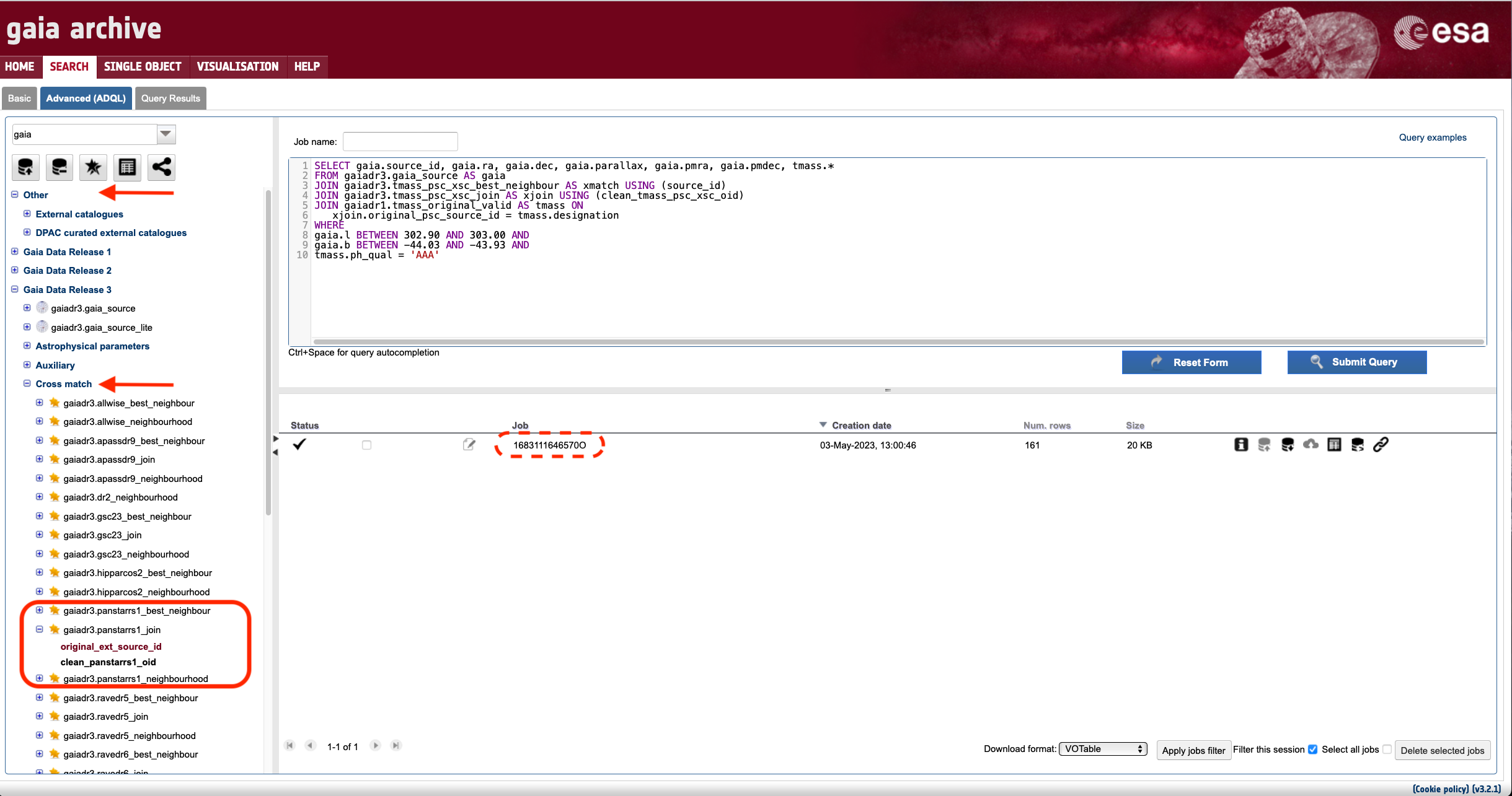
Figure 1: Excerpt of the Advanced (ADQL) tab in the Gaia Aerchive web interface. The top arrow points to the "Other" namespace that contains external and DPAC-curated catalogues. Most of them can be used in combination with the pre-computed cross-matches generated for each Gaia release that are listed under "Cross match" namespace (highlighted by the bottom arrow). The tables generated for the PanSTARRS-DR1 catalogue are encompassed by the large rectangle. The Job ID of the query executed in the ADQL query editor (see the Advanced ADQL tutorial for more details) is highlighted by the small rectangle.
Two complementary tables are provided for each cross-matched catalogue: the "_best_neighbour" and "_neighbourhood" tables (e.g., "gaiaedr3.panstarrs1_best_neighbour" and "gaiaedr3.panstarrs1_neighbourhood", see Fig.1). Since Gaia EDR3, an extra "_join" table is included for most cross-matches (e.g., "gaiaedr3.panstarrs1_join"). This table was introduced to facilitate the analysis of the cross-match outcome when several sources are matched to the same Gaia source. In this case, using the "_join" table, it is possible to retrieve all the multiple matches by means of its "clean_<catalogue_name>_oid" field. Most importantly, since Gaia EDR3 the pre-computed cross-match with the 2MASS catalogue merges the Point Source Catalogue (2MASS PSC) and Extended Source Catalogue (2MASS XSC). Using the "gaiaedr3.tmass_psc_xsc_join" table (via its "original_psc_source_id" and "original_xsc_source_id" fields) is therefore mandatory to properly use this pre-computed cross-match. Finally, Gaia EDR3 also includes a pre-computed cross-match to the Gaia DR2 main catalogue.
This intermediate-level tutorial explains how to use the cross-matches included in the Gaia Early Data Release 3. Nevertheless, the examples listed below can be extended to previous data releases as long as the differences in the pre-computed cross-matches are considered. In case of difficulties following this exercise, please take a look at the introductory tutorials Basic queries and Advanced (ADQL) queries.
Tutorial Content:
1. Input Samples
The first step of this exercise is creating the samples that are going to be cross-matched in the forward (Gaia catalogue >> external catalogue) and backward (external catalogue >> Gaia catalogue) directions. To do so we retrieve all sources contained in a circle (radius = 0.5 degrees) centred in Baade's Window (ra = 270.89 deg, dec = -30.03 deg) from the Gaia EDR3, PanSTARRS-DR1, and the 2MASS PSC catalogues. After completion, the query results are uploaded to the user space as explained in this tutorial.
1.1 GAIA EDR3
SELECT source_id, ra, dec, parallax, pmra, pmdec, phot_g_mean_mag, phot_bp_mean_mag, phot_rp_mean_mag
FROM gaiaedr3.gaia_source
WHERE DISTANCE(POINT(270.89, -30.03),POINT(ra, dec)) < 0.5
-- Extra filter to retrieve the sources having the most reliable astrometric parameters
AND ruwe < 1.4
Output = 358,976 sources. Uploaded to the user space as: "user_hcanovas.baade_edr3".
1.2 2MASS PSC
SELECT tmass_oid, designation, ra, dec, err_maj, err_min, j_m
FROM gaiadr1.tmass_original_valid
WHERE DISTANCE(POINT(270.89, -30.03), POINT(ra, dec)) <0.5
Output = 87,903 sources. Uploaded to the user space as: "user_hcanovas.baade_twomass".
1.3 PANSTARRS-DR1
SELECT obj_name, obj_id, ra, dec, epoch_mean, g_mean_psf_mag, r_mean_psf_mag, i_mean_psf_mag
FROM gaiadr2.panstarrs1_original_valid
WHERE DISTANCE(POINT(270.89, -30.03), POINT(ra, dec)) < 0.5
Output = 658,536 sources. Uploaded to the user space as: "user_hcanovas.baade_ps1".
2. 2mass
2.1 forward direction
The examples below show how to retrieve the 2MASS PSC counterparts of the Gaia EDR3 sample created in Sect. 1.1.
2.1.1 siNGLE cross-match
Only the matched source with better astrometry in the 2MASS PSC catalogue is included in the query outcome:
SELECT gaia.source_id, gaia.ra, gaia.dec, gaia.parallax, xmatch.original_ext_source_id,
xmatch.clean_tmass_psc_xsc_oid, tmass.ra AS ra_tm, tmass.dec AS dec_tm, err_maj, err_min, tmass.tmass_oid, tmass.designation, xmatch.angular_distance
FROM user_hcanovas.baade_edr3 AS gaia
JOIN gaiaedr3.tmass_psc_xsc_best_neighbour AS xmatch USING (source_id)
JOIN gaiaedr3.tmass_psc_xsc_join AS xjoin
  ON xmatch.original_ext_source_id = xjoin.original_psc_source_id
JOIN gaiadr1.tmass_original_valid AS tmass
  ON xjoin.original_psc_source_id = tmass.designation
ORDER BY gaia.dec ASC
Output = 66,495 sources. Execution time ~ 10 seconds.
2.1.2 MULTI cross-match
All matches are retrieved. This is accomplished by targeting the "clean_tmass_psc_xsc_oid" field in the "gaiaedr3.tmass_psc_xsc_join" table (instead of the "original_psc_source_id" field used in the previous example):
SELECT gaia.source_id, gaia.ra, gaia.dec, gaia.parallax, xmatch.original_ext_source_id, xmatch.clean_tmass_psc_xsc_oid,
tmass.ra AS ra_tm, tmass.dec AS dec_tm, err_maj, err_min, tmass.tmass_oid, tmass.designation, xmatch.angular_distance
FROM user_hcanovas.baade_edr3 AS gaia
JOIN gaiaedr3.tmass_psc_xsc_best_neighbour AS xmatch USING (source_id)
JOIN gaiaedr3.tmass_psc_xsc_join AS xjoin USING (clean_tmass_psc_xsc_oid)
JOIN gaiadr1.tmass_original_valid AS tmass
  ON xjoin.original_psc_source_id = tmass.designation
ORDER BY gaia.dec ASC
Output = 66,498 sources. Execution time ~ 10 seconds.
This query produces 3 more sources than the "single" cross-match. This means that our Gaia EDR3 sample contains sources having multiple matches in the 2MASS PSC catalogue. The previous query has job_id = 1641819319674O. Using the job_upload functionality it is possible to identify these sources as follows:
SELECT source_id, COUNT(source_id) AS n_reps
FROM job_upload."job1641819319674O"
GROUP BY source_idHAVING COUNT(source_id) > 1
Output = 3 sources. Execution time ~ 5 seconds.
This output contains 3 Gaia EDR3 sources, each one having two matches in the 2MASS PSC catalogue. The previous query has job_id = 1641819972509O. As before, we can use the job_upload functionality to inspect the properties of these multiple matches:
SELECT * FROM job_upload."job1641819319674O"
JOIN job_upload."job1641819972509O" USING (source_id)
Output = 6 sources. Execution time ~ 5 seconds. An excerpt of the output of this query is shown in Fig. 2.
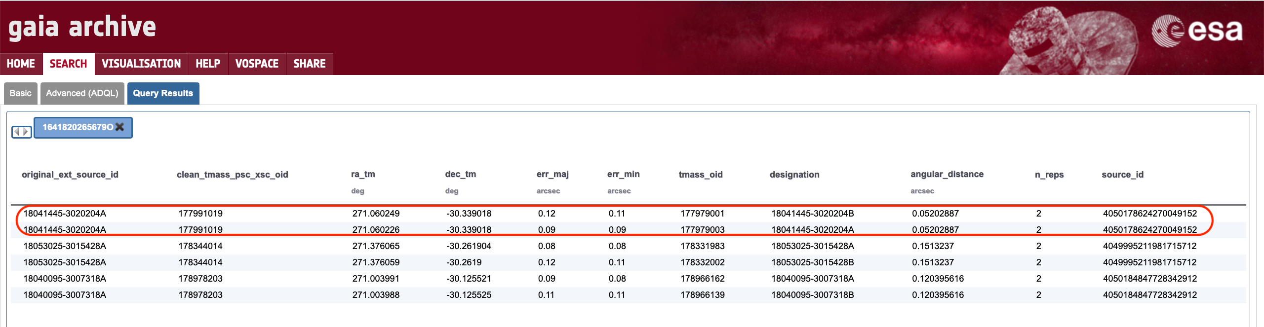
Figure 2: Results of the last query displayed above. Each Gaia EDR3 source has two matches in the 2MASS PSC catalogue. For example, the source 4050178624270049152 is matched by 18041445-3020204A and 18041445-3020204B (see the "designation" column) in the 2MASS PSC catalogue.
For comparison, source 4050178624270049152 is only matched to 18041445-3020204A (which has better astrometry than 18041445-3020204B) in the "single cross-match" described in Sect. 2.1.1 above.
2.2 Backwards DIRECTION
The examples below show how to retrieve the Gaia EDR3 counterparts of the 2MASS PSC sample created in Sect. 1.2
2.2.1 siNGle cross-match
As in Sect. 2.1.1 above, only the source with better astrometry in the 2MASS PSC catalogue is included in the query outcome in case of multiple matches.
SELECT gaia.source_id, gaia.ra, gaia.dec, gaia.parallax, xmatch.original_ext_source_id, xmatch.clean_tmass_psc_xsc_oid,
tmass.ra AS ra_tm, tmass.dec AS dec_tm, err_maj, err_min, tmass.tmass_oid, tmass.designation, xmatch.angular_distance
FROM user_hcanovas.baade_twomass AS tmass
JOIN gaiaedr3.tmass_psc_xsc_join AS xjoin
  ON xjoin.original_psc_source_id = tmass.designation
JOIN gaiaedr3.tmass_psc_xsc_best_neighbour AS xmatch
  ON xmatch.original_ext_source_id = xjoin.original_psc_source_id
JOIN gaiaedr3.gaia_source AS gaia USING (source_id)
WHERE ruwe < 1.4
ORDER BY gaia.dec ASC
Output = 66,492. Execution time ~ 10 seconds.
2.2.2 MULTI cross-match
All matches are retrieved.
SELECT gaia.source_id, gaia.ra, gaia.dec, gaia.parallax, xmatch.original_ext_source_id, xmatch.clean_tmass_psc_xsc_oid,
tmass.ra AS ra_tm, tmass.dec AS dec_tm, err_maj, err_min, tmass.tmass_oid, tmass.designation, xmatch.angular_distance
FROM user_hcanovas.baade_twomass AS tmass
JOIN gaiaedr3.tmass_psc_xsc_join AS xjoin
  ON xjoin.original_psc_source_id = tmass.designation
JOIN gaiaedr3.tmass_psc_xsc_best_neighbour AS xmatch USING (clean_tmass_psc_xsc_oid)
JOIN gaiaedr3.gaia_source AS gaia USING (source_id)
WHERE ruwe < 1.4
ORDER BY gaia.dec ASC
Output = 66,495. Execution time ~ 10 seconds.
3. panstarrs-dr1
3.1 FORward direction
The examples below show how to retrieve the PanSTARRS-DR1 counterparts of the Gaia EDR3 sample created in Sect. 1.1.
3.1.1 siNGLE cross-match
Only the matched source with better astrometry in the PanSTARRS-DR1 catalogue is included in the outcome of the query:
SELECT gaia.source_id, gaia.ra, gaia.dec, gaia.parallax, xmatch.original_ext_source_id, xmatch.clean_panstarrs1_oid,
psdr1.ra AS ra_ps, ra_error, psdr1.dec AS dec_ps, dec_error, psdr1.obj_name, psdr1.obj_id, xmatch.angular_distance,
g_mean_psf_mag, r_mean_psf_mag, i_mean_psf_mag
FROM user_hcanovas.baade_edr3 AS gaia
JOIN gaiaedr3.panstarrs1_best_neighbour AS xmatch USING (source_id)
JOIN gaiadr2.panstarrs1_original_valid AS psdr1
   ON xmatch.original_ext_source_id = psdr1.obj_id
ORDER BY gaia.dec ASC
Output = 271,105 sources. Execution time ~ 15 seconds.
REMEMBER: the join operation with the "gaiaedr3.panstarrs1_join" table is not needed in the single cross-match case unless the cross-match is performed with the 2MASS catalogue (as in Sects. 2.1.1 and 2.2.1 above), as in this case the pre-computed tables contain data from the Point Source (2MASS PSC) and Extended Source (2MASS XSC) catalogues.
3.1.2 Multi cross-match
All matches are retrieved. This is accomplished by targeting the "clean_panstarrs1_oid" field in the "gaiaedr3.panstarrs1_join" table:
SELECT gaia.source_id, gaia.ra, gaia.dec, gaia.parallax, xjoin.original_ext_source_id, xjoin.clean_panstarrs1_oid, psdr1.ra AS ra_ps,
ra_error, psdr1.dec AS dec_ps, dec_error, psdr1.obj_name, psdr1.obj_id, xmatch.angular_distance, g_mean_psf_mag, r_mean_psf_mag, i_mean_psf_mag
FROM user_hcanovas.baade_edr3 AS gaia
JOIN gaiaedr3.panstarrs1_best_neighbour AS xmatch USING (source_id)
JOIN gaiaedr3.panstarrs1_join AS xjoin USING (clean_panstarrs1_oid)
JOIN gaiadr2.panstarrs1_original_valid AS psdr1
   ON xjoin.original_ext_source_id = psdr1.obj_id
ORDER BY gaia.dec ASC
Output = 272,680 sources. Execution time ~ 20 seconds.
Please take a moment to examine this result and compare it with the previous one. The output of this query indicates that there are 272,680 - 271,105 = 1,575 multiple matches. Those can be easily identified (and inspected) following the steps detailed in Sect. 2.1.2.
3.2 Backward direction
The examples below show how to retrieve the Gaia EDR3 counterparts of the PanSTARRS-DR1 sample created in Sect. 1.3.
3.2.1 siNGLE cross-match
SELECT gaia.source_id, gaia.ra, gaia.dec, gaia.parallax, psdr1.ra AS ra_ps, psdr1.dec AS dec_ps, obj_name, obj_id, angular_distance, g_mean_psf_mag, r_mean_psf_mag, i_mean_psf_mag
FROM user_hcanovas.baade_ps1 AS psdr1
JOIN gaiaedr3.panstarrs1_best_neighbour AS xmatch
  ON xmatch.original_ext_source_id = psdr1.obj_id
JOIN gaiaedr3.gaia_source AS gaia USING (source_id)
WHERE ruwe < 1.4
ORDER BY gaia.dec ASC
Output = 271,107 sources. Execution time ~ 20 seconds.
3.2.2 Multi cross-match
All matches are retrieved. As in Sect. 3.1.2 above, this is accomplished by targeting the "clean_panstarrs1_oid" field in the "gaiaedr3.panstarrs1_join" table:
SELECT gaia.source_id, gaia.ra, gaia.dec, gaia.parallax, xjoin.original_ext_source_id, xjoin.clean_panstarrs1_oid, psdr1.ra AS ra_ps,
psdr1.dec AS dec_ps, obj_name, obj_id, angular_distance, g_mean_psf_mag, r_mean_psf_mag, i_mean_psf_mag
FROM user_hcanovas.baade_ps1 AS psdr1
JOIN gaiaedr3.panstarrs1_join AS xjoin
   ON xjoin.original_ext_source_id = psdr1.obj_id
JOIN gaiaedr3.panstarrs1_best_neighbour USING (clean_panstarrs1_oid)
JOIN gaiaedr3.gaia_source AS gaia USING (source_id)
WHERE ruwe < 1.4
ORDER BY gaia.dec ASC
Output = 272,681 sources. Execution time ~ 20 seconds.
As in the forward cross-match (Sect. 3.1), this result indicates that there are 272,681 - 271,107 = 1,574 multiple matches. Those can be easily identified (and inspected) following the steps detailed in Sect. 2.1.2.
4. Gaia DR2
The "gaiaedr3.dr2_neighbourhood" table inside the "Auxiliary" name space in the tables tree (see Fig. 1 above) allows to identify Gaia DR2 sources in the Gaia EDR3 catalogue (and vice versa). This table was created by applying a simple linear proper-motion correction (when possible) to all Gaia EDR3 objects and looking for Gaia DR2 matches within a 2” radius - see Chapter 10 of the Gaia EDR3 documentation for a thorough description of the motivation and creation details of this table. Below, we show how to retrieve the Gaia DR2 sources matched to the Gaia EDR3 sample created in Sect. 1.1:
SELECT gaiaedr3.*, dr2toedr3.*
FROM user_hcanovas.baade_edr3 AS gaiaedr3
JOIN gaiaedr3.dr2_neighbourhood AS dr2toedr3
   ON dr2toedr3.dr3_source_id = gaiaedr3.source_id
ORDER BY gaiaedr3.ra ASC
Output = 554,805 sources. Execution time ~ 20 seconds.
A quick comparison with the input EDR3 sample (which contains 358,976 sources) reveals that a significant fraction of the outcome of this query contains multiple matches. This is a consequence of the extreme stellar density of the region that is being analysed (Baade's window). The fraction of multiple matches can be easily reduced by applying additional filters to the query, for example:
SELECT gaiaedr3.*, dr2toedr3.*
FROM user_hcanovas.baade_edr3 AS gaiaedr3
JOIN gaiaedr3.dr2_neighbourhood AS dr2toedr3
   ON dr2toedr3.dr3_source_id = gaiaedr3.source_id
-- Exclude sources having G-band magnitude differences above 0.1 mag
WHERE ABS(magnitude_difference) < 0.1
ORDER BY gaiaedr3.ra ASC
Output = 337,641 sources. Execution time ~ 20 seconds.
- Removed a total of (5) style text-align:center;
- Removed a total of (17) style text-align:justify;
- Removed a total of (2) style margin:0;
Tutorial: catalogue combination
Authors: Héctor Cánovas, Jos de Bruijne, and Alcione Mora
One of the most popular Frequently Asked Questions to the Archive Helpdesk is how to combine Gaia data with other catalogues. The simplest way to do this, provided that the target catalogue shares at least one common field such as the source identifier, is using the ADQL JOIN operation. Otherwise, a geometrical match with a Cone Search will be needed. In this case, it is important to recognise that cross-matching catalogues is a non-trivial, scientific exercise. That is, there are no general rules to determine whether two observations made by different telescopes and/or instruments, at different wavelengths, with a different (spatial) resolution, at a different epoch, etc. are physically related to the same object. This decision depends on the context and science case at hand and can only be addressed by the astronomer asking the question. For example, some Gaia EDR3 sources (visible, sub-arcsecond resolution, epoch J2016) might be related to IRAS 100 micrometre photometry (far-infrared, 2- arcminute resolution, epoch 1983) for the purpose of constructing Spectral Energy Distributions of pre-main sequence stars surrounded by circumstellar discs. However, VLBI coeval quasar astrometry needs careful combination with Gaia when comparing ICRF and Gaia-CRF realisations, due to possible microarcsecond offsets between the radio and visible emitting regions, see e.g. Mignard+ (2018). Having said that, there are tips that can help us in this endeavour. To begin with, the most important tools are the geometrical conditions that identify potential matches between sources based on their projected separation on the celestial sphere. However, proximity alone is not a match guarantee and it should be supplemented by adding additional constraints in, e.g., flux and/or parallax. Finally, proper motions and other parameters need to be taken into account for fast-moving objects when the time difference between catalogues is considerable.
The Gaia ESA Archive hosts copies of several major surveys and catalogues. Some of them have been curated by DPAC (see Chapters 9, 13.2, and 13.3 in the Gaia EDR3 Documentation, and also Chapters 10.9, 14.4, and 14.5 of the Gaia DR2 Documentation and Chapters 3 and 4 of the Gaia DR1 Datamodel description), while others have been directly copied or adapted from external archives (e.g. external.apassdr9, public.hipparcos_newreduction). They can be found in the tables tree under the branch "Other". Furthermore, registered users of the Gaia ESA Archive can upload their own catalogues to their user space, where they can store up to 1 GB of tabular data.
This intermediate level tutorial introduces the basic concepts needed to combine catalogues (either uploaded by registered users or hosted by the Archive) using the Advanced (ADQL) tab. The introductory tutorials Basic queries, Advanced (ADQL) tab, and Upload a user table should be read first in case of difficulties following this exercise. Novice users migh be interested in learning how to run a cross-match between a very small (<2000 entries) input target list and any of the catalogues accessible through the Basic form (as shown in this tutorial), while advanced users aiming to learn how to include the epoch propagation are adviced to look at this tutorial. Finally, please keep in mind that the Archive contains DPAC-curated cross-matches between the main Gaia catalogues and many of the most popular astronomical surveys. We recommend to use these pre-computed cross-matches whenever possible, as explained in this tutorial. Users interested in retrieving ALL matches from two large catalogues (e.g., 2MASS and the main catalogue of Gaia EDR3) are strongly adviced to NOT use the Archive, but instead download the catalogues in bulk (here - see also this FAQ) for off-line analysis.
Tutorial Content:
1. JOINing catalogues
If the target catalogues contain at least one field in common like, e.g., source_id or designation, combining them using the JOIN ADQL clause is nearly trivial. There are, however, some caveats worth to be considered before bluntly applying the JOIN statement. First of all, the default ADQL JOIN operation is the INNER JOIN (that only returns the common elements between the joined catalogues), but there are a number of JOIN types that return very different outputs (see, e.g., the JOIN SQL Apache documentation). Second, users must be careful when combining the JOIN with the WHERE SQL clause, as suboptimal queries can easily yield to a time-out. For example, the following query shows how to (optimally) combine two catalogues to extract a sample that complies with two different filters:
SELECT G.*, B.*
FROM gaiaedr3.gaia_source AS G
JOIN external.gaiaedr3_distance AS B USING (source_id)
-- Conditions: ==================
WHERE G.dr2_radial_velocity IS NOT NULL
AND B.r_med_geo > 20000
Output: 1503 records. Execution time ~30 seconds.
The following sub-optimal query, although being conceptually similar, will time-out:
SELECT G.*, B.* FROM gaiaedr3.gaia_source AS G, external.gaiaedr3_distance AS B
WHERE G.dr2_radial_velocity IS NOT NULL
AND B.r_med_geo > 20000
2. Cross-matching catalogues (basic)
2.1 Introduction
Before executing an ADQL Cone Search, it is important to make sure that the details of this operation are well understood. On the one hand, the astrometry of the combined catalogues should be provided in the same reference system. The Gaia astrometry is consistently given in the International Celestial Reference System (ICRS). On the other hand, it is possible (and even likely) that the reference epoch to which the celestial coordinates are referred is different in the catalogues being cross-matched. For example, when cross-matching Gaia EDR3 astrometry (which is provided at epoch J2016.0) with a catalogue having astrometry at epoch J2000.0, the Cone Search radius should be large enough to encompass the coordinate shifts caused by the proper motion of the sources in the sky during the 16-year interval. Even without a priori knowledge of the proper motions of the target sources in a cross-match, we can proceed as follows to estimate the radius that should be used in the Cone Search. Most sources in the Gaia EDR3 main catalogue move slowly (below 50 mas/yr), as shown by the following query:
SELECT source_id, ra, dec, parallax, pmra, pmdec, pm, dr2_radial_velocity, ref_epoch
FROM gaiaedr3.gaia_source
WHERE pm > 50
Output: 3,273,397 records.
This means that the vast majority of the main EDR3 catalogue (which contains ~1.8 billion sources, so 99.8% of it) moves less than 5 arcsec per century. Therefore, unless the cross-match includes high-proper-motion stars, we can safely use the following approach:
radiuscone_search = 1" + δ epoch [yr] x 0.050"/yr
where a tolerance of 1" is used to account for the potential astrometric uncertainties between catalogues, and "δ epoch [yr]" is the time interval between the reference epochs of the cross-matched catalogues (16 years in the previous example).
In the following examples, we describe how to combine a small (<100,000 entries), user-defined catalogue with any catalogue hosted by the Archive. The first step is to retrieve the data that will serve as the external catalogue to be cross-matched. We will use the HST/ACS photometry from the NGC 346 open cluster analysed by Gouliermis+ (2006), that contains data for 99,079 sources. It can be retrieved following the steps described in the external TAP tutorial or, alternatively, by clicking on this link and pressing on the "Submit" after loading the VizieR page. In both cases, the output can be uploaded to the Gaia ESA Archive user space while authenticated, as explained in this tutorial. For this example, we will name the table as "gouliermis_2006", so once uploaded to our user space, its name in the Archive is "user_hcanovas.gouliermis_2006". Note that in order to replicate the following queries, the table name "user_hcanovas.gouliermis_2006" should be replaced by "user_<your_user_name>.gouliermis_2006". Following the approach outlined above, the Cone Search radius for this example will be set as: radiuscone_search = 1" + 16 yr x 0.050"/yr = 1.8".
2.2 ADQL Cone Search
The most basic (and powerful) geometric ADQL condition is the Cone Search, which is a particular case of a geometric cross-match (see the IVOA recommended implementation of the Cone Search). It selects potential matches based on angular proximity. We recommend you take your time to learn it. In many cases, this restriction alone is what most astronomers need. The following query cross-matches the uploaded catalogue against Gaia EDR3 using a 1 arcsec Cone Search radius (note that the radius unit is fixed to degrees so that a conversion from arcseconds to degrees is needed in the query):
SELECT num, source_id, ra, dec, parallax, pmra, pmdec, vmag, imag, phot_g_mean_mag, phot_bp_mean_mag, phot_rp_mean_mag, DISTANCE(POINT(raj2000, dej2000), POINT(ra, dec) ) * 3600. AS dist_arcsec
FROM user_hcanovas.gouliermis_2006 AS gouliermis
-- Geometric Cross-Match: =======
JOIN gaiaedr3.gaia_source AS gaia
  ON DISTANCE(POINT(raj2000, dej2000),POINT(ra, dec)) <1.8 / 3600.
Output: 73,492 records. Note: the geometrical condition is applied in the JOIN (match) between tables: circles of 1.8 arcsec (1.8 deg / 3600.) are traced around objects in the main Gaia catalogue to look for sources in the external catalogue.
2.3 Archive Built-in tool
A built-in cross-match tool is available for authenticated users. It produces a simple Cone Search (as in Sect. 2.2 above) and it might be a good starting point for users with little experience in ADQL. The first step is to update the metadata of the (uploaded) table to identify the Ra and Dec columns, as explained in the Upload a user table tutorial (see its Fig. 4). Once this is done, the table icon will resemble a celestial sphere (see the tables tree in Fig. 1).
Next, click on the double-star icon placed on top of the tables tree to launch the built-in cross-match tool (see Fig. 1, red circle on top of the tables tree). A pop-up window will open, allowing to select the input table, the target catalogue, and the cross-match radius. Clicking on the "Execute" button will produce the user table "user_hcanovas.xmatch_gouliermis_2006_gaia_source" with the cross-match and the empty job xmatch_gouliermis_2006_gaia_source (first job in the Job lists area shown in Fig. 1). Clicking on the "Join" icon of that job (highlighted by a red circle in Fig. 1) generates the final join query between Gouliermis+ (2006), Gaia, and the cross-match table. This ADQL query will appear in the ADQL query editor box.
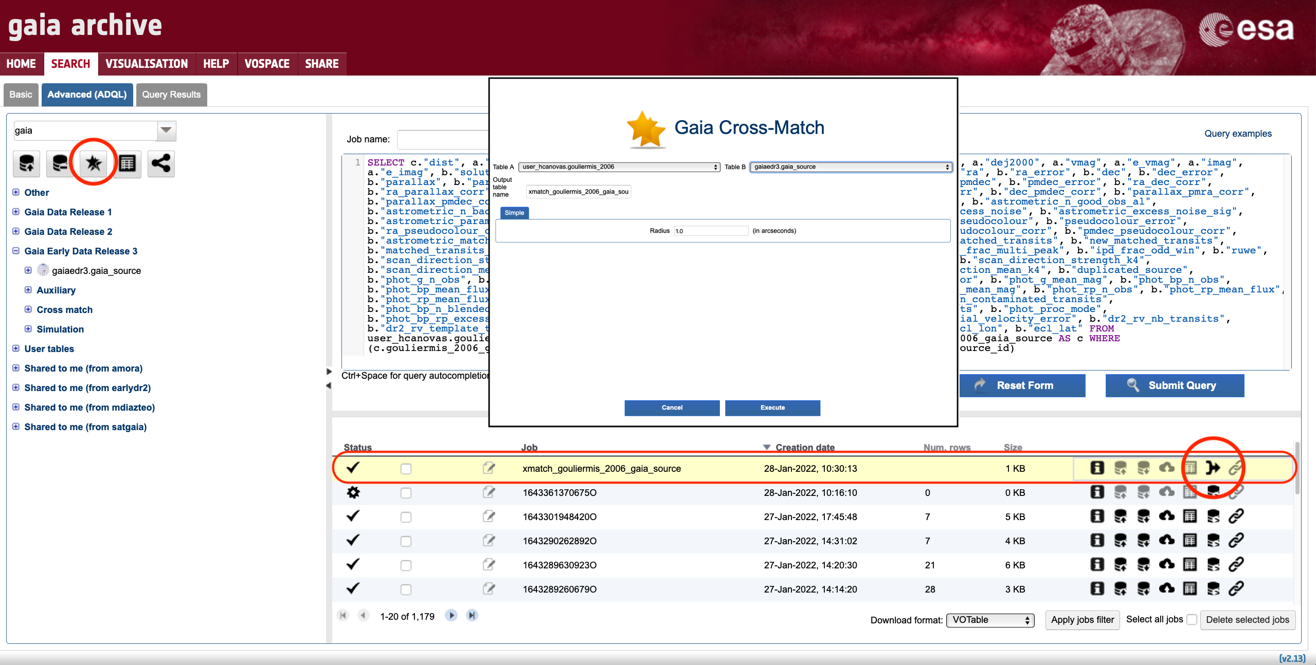
Figure 1: Different steps of the built-in cross-match. First, click on the double-star icon (encompassed by the red circle on the left side of the panel). A pop-up window that allows to choose the tables to be cross-matched will show-up. Once the cross-match is executed, it will appear in the job list panel (as highlighted by the large red rectangle). This is an intermediate job. In order to produce the final results of the cross-match, click on the "Show join query" icon encompassed by the red circle on the right side of the panel. The ADQL query will load in the ADQL Query editor. Finally, press the "Submit Query" buttom to execute the query and generate the cross-match results.
In the example below, the query has been edited to retrieve only a few columns:
SELECT c."separation",  a."num", a."vmag", a."imag",  b."source_id", b."ra", b."dec", b."parallax", b."pmra", b."pmdec", b."phot_g_mean_mag", b."phot_bp_mean_mag", b."phot_rp_mean_mag"
FROM user_hcanovas.gouliermis_2006 AS a, gaiaedr3.gaia_source AS b, user_hcanovas.xmatch_gouliermis_2006_gaia_source AS c
WHERE (c.gouliermis_2006_gouliermis_2006_oid = a.gouliermis_2006_oid  AND c.gaia_source_source_id = b.source_id)
3. Cross-matching catalogues (advanced)
As explained in the introduction, cross-matches are scientific problems and additional insight (in the form of extra constraints or filters) is usually needed on top of a basic Cone Search. Furthermore, sometimes we are interested in gathering the data contained across more than one catalogue. The examples below show how to create these advanced cross-matches.
3.1 ADQL Cone Search + extra condition
The following query adds an extra photometric condition to the query shown in Sect. 2.2 by enforcing |V - G| < 2 mag, which is a reasonable filter to reduce the number of false positives due to the similarity in wavelength and spatial resolution of Gaia and HST/ACS. This condition is particularly effective due to the HST/ACS catalogue containing several crowded areas (stellar clusters and associations).
SELECT num, source_id, ra, dec, parallax, pmra, pmdec, vmag, imag, phot_g_mean_mag, phot_bp_mean_mag, phot_rp_mean_mag, DISTANCE(POINT(raj2000, dej2000),POINT(ra, dec) ) * 3600. AS dist_arcsec
FROM user_hcanovas.gouliermis_2006 AS gouliermis
-- Geometric Cross-Match: =======
JOIN gaiaedr3.gaia_source AS gaia
  ON DISTANCE(POINT(raj2000, dej2000),POINT(ra, dec)) <1.8 / 3600.
-- Condition: ===================
WHERE ABS(vmag - phot_g_mean_mag) < 2.
Output: 12,100 records. Note: the photometric condition reduces the number of possible matches by a factor ~6 compared to the previous result in Sect. 2.2.
3.2 ADQL Cone Search + extra condition + join (Two large tables)
Imagine we are only interested in matches simultaneously having Gaia DR2 and Gaia EDR3 counterparts. This would translate into combining three tables: Gouliermis+ (2006) for the HST/ACS photometry, "gaiaedr3.gaia_source" for the astrometry and photometry, and "gaiaedr3.dr2_neighbourhood" for the Gaia DR2 - Gaia EDR3 cross-match. This means that three tables need to be combined (joined) together. The first question to answer is: can it be done in consecutive steps? In other words: could we combine the HST/ACS with Gaia EDR3 data first, and then add the second cross-match+filter to remove the unlikely matches? We recommend to proceed in this way whenever possible, as it is advantageous in terms of performance. Let us assume that the results obtained above in Sect. 3.1 produce a job with ID 1618840042709O. These results, being small, could be reused by using either JOB_UPLOAD or uploading the intermediate table to the user space. In the example below, we use the pre-computed DR2-EDR3 cross-match (see Chapter 10 of the Gaia EDR3 documentation) available in the Archive to combine the third catalogue, and add an extra photometric condition to that match:
SELECT intermediate.*, dr3Xdr2.*
FROM job_upload."job1618840042709O" AS intermediate
-- 2nd Match: ===================
JOIN gaiaedr3.dr2_neighbourhood AS dr3Xdr2 ON dr3xdr2.dr3_source_id = source_id
-- 2nd Extra condition: =========
WHERE ABS(magnitude_difference) < 0.1
Output: 6,798 records.
Note that in this example the third catalogue is added using a JOIN operation, as the combined catalogues have one field in common (the source ID in the Gaia EDR3 main catalogue). Would that not be the case, a geometrical cross-match as implemented in Sect. 2.2 above could be used.
There are many situations where the two-step process explained above is impossible or undesirable. For example, if the intermediate table is very large. In these cases, the query can be divided into different steps. First, use a subquery to isolate whatever block needs to be executed earlier (typically the geometrical condition). Then, add the "OFFSET 0" clause at the end of the subquery. This condition has no semantic meaning (it does not skip any records). However, it instructs the Archive PostgreSQL data base backend to respect the logical order (the subquery is executed first and other conditions applied afterwards). Let us see an example:
SELECT * FROM (
     SELECT * FROM (
      SELECT Num, source_id, ra, dec, parallax, pmra, pmdec, Vmag, Imag, phot_g_mean_mag, phot_bp_mean_mag, phot_rp_mean_mag
      FROM user_hcanovas.gouliermis_2006 AS gouliermis
      -- Geometric condition: ===============
      JOIN gaiaedr3.gaia_source AS gaia
          ON DISTANCE(POINT(raj2000, dej2000), POINT(ra, dec)) <1.8 / 3600.     OFFSET 0 ) AS subquery
      -- DR2xDR3 CrossMatch =================
    JOIN gaiaedr3.dr2_neighbourhood AS dr3xdr2
       ON dr3xdr2.dr2_source_id = source_id   OFFSET 0 ) AS subquery2
      -- Extra conditions: ==================
  WHERE ABS(Vmag - phot_g_mean_mag) < 2. AND
  ABS(magnitude_difference) < 0.1
It uses two subqueries with OFFSET 0 to enforce the following logical sequence: Cone Search => join to Gaia DR2 X Gaia EDR3 cross-match table => photometric conditions. The resulting query is elegant, and produces all the results in one go. However, it takes more execution time than splitting the query into two separate jobs (~40 minutes versus a few seconds).
- Removed a total of (1) style text-align:center;
- Removed a total of (38) style text-align:justify;
- Removed a total of (1) style margin:0;
- Removed a total of (1) style display:none;
Proper-motion corrected cross-match. Introduction
Author: Alcione Mora
Stars move in the sky. This means the full astrometry (mostly proper motions) needs to be considered when cross-matching catalogues with fast moving objects separated by a significant time difference. In addition, reference systems also evolve, as our knowledge of the sky improves. For example, the Gaia DR1 and DR2 Celestial Reference Frames are different, see Mignard+ (2018) .
In any case, the science case drives the level of detail. In many situations, astronomers are only interested in lists of potential matches, and arcsec level position tolerance is acceptable. This is the focus for the remainder of this tutorial.
A more careful work is needed to e.g. determine long baseline proper motions or accelerations. This is outside the scope of this tutorial. See e.g. Brandt (2018) for a recent comparison between Hipparcos and Gaia DR2.
The first thing to consider is most stars move very slowly. Gaia DR2 contains slightly less than 1 million stars moving faster than 50 mas/yr, as shown by the following query.
select source_id, ra, dec, parallax, pmra, pmdec, sqrt(pmra * pmra + pmdec * pmdec) as pm, radial_velocity, ref_epoch from gaiadr2.gaia_source where (pmra < -50 / sqrt(2) or pmra > 50 / sqrt(2)) and (pmdec < -50 / sqrt(2) or pmdec > 50 / sqrt(2)) and sqrt(pmra * pmra + pmdec * pmdec) > 50
Output: 976538 records
This means the bulk of the catalogue (1.3 billion) moves less than 5 arcsec per century. Should the objects of interest belong to this group, cross-match candidates could be selected just enlarging the cone search radius appropriately.
Proper-motion enlarged cross-match. USNO B1 vs Gaia, M4 globular cluster
Imagine we want to combine USNO B1 photometry with Gaia DR2 in a circle of 0.5 deg centred around the globular cluster M4, which has a small proper motion. This external catalogue can be explored as an external TAP. Using keywords "usno b1", reveals two copies at CDS and IRSA. If the former is selected, the following query retrieves the data
select "USNO-B1.0", "Tycho-2", raj2000, dej2000, epoch, pmra, pmde, mupr, b1mag, r1mag, b2mag, r2mag from "I/284/out" where 1 = contains( point('ICRS', raj2000, dej2000), circle('ICRS', 245.89675000000003, -26.52575, 0.5) )
Output: 43060 records
Statistics on the observation epoch can be retrieved analysing the output with JOB_UPLOAD (job ID for this exercise: 1564403845697O). Remember to switch back to the Gaia Archive to reuse jobs.
select min(epoch), max(epoch), avg(epoch) from job_upload."job1564403845697O"

The first epoch in the M4 sample is thus 1954.2. Imagine we want a cone search including all neighbours that have been closer than 2 arcsec, irrespective of the observation epoch. The cross-match radius between Gaia and M4 can be estimated as follows: 2 arcsec (tolerance) + 50 mas/yr (maximum proper motion for slow stars) * (2015.5 – 1954.2) yr = 5.0 arcsec. A first list of potential Gaia DR2 - USNO B1 matches can be obtained using such a cross-match radius. JOB_UPLOAD will be used to upload the previous USNO results (job ID 1564407875966O) and compare them to gaia_source.
select usno.*, gaia.source_id, gaia.ra, gaia.dec, gaia.parallax, gaia.pmra as pmra_gaia, gaia.pmdec as pmdec_gaia, radial_velocity, phot_g_mean_mag, phot_bp_mean_mag, phot_rp_mean_mag from job_upload."job1564407875966O" as usno join gaiadr2.gaia_source as gaia on 1 = contains( point(usno.raj2000, usno.dej2000), circle(gaia.ra, gaia.dec, 5. / 3600.) )
Output: 80410 records
Such query (job ID job1564413301477O) contains all potential matches between both catalogues, and might be enough for many users intending to select the good matches a posteriori on their computers.
Proper-motion enlarged cross-match. USNO B1 vs Gaia, high proper motion stars
Imagine we are interested on the fastest moving objects in Gaia. This is the complementary exercise to the previous section. For simplicity, only objects faster than 2 arcsec/yr will be considered. The sample can be selected using the following query.
select source_id, ra, dec, parallax, pmra, pmdec, sqrt(pmra * pmra + pmdec * pmdec) as pm, radial_velocity, ref_epoch from gaiadr2.gaia_source where (pmra < -2000 / sqrt(2) or pmra > 2000 / sqrt(2)) and (pmdec < -2000 / sqrt(2) or pmdec > 2000 / sqrt(2)) and sqrt(pmra * pmra + pmdec * pmdec) > 2000 order by pm desc
Output: 28 records
The highest proper motion corresponds to Barnard's star: 10.4 arcsec/yr. If the earliest epoch in USNO B1 of 1949 is considered, see Monet+ (2003), the search radius can be estimated as 2 arcsec + 10.4 arcsec/yr * (2015.5 - 1949) = 693.6 arcsec = 11.5 arcmin. The following query in the external Archive TAP-Vizier (remember to switch) can be requested from the Gaia Archive using TAP_UPLOAD (job ID 1564409893418O) to provide the high proper motion Gaia stars and retrieve potential matches
select "USNO-B1.0", "Tycho-2", raj2000, dej2000, epoch, usno.pmra, usno.pmde, usno.mupr, b1mag, r1mag, b2mag, r2mag, gaia.* from "I/284/out" as usno join TAP_UPLOAD.JOB1564409893418O as gaia on 1 = contains( point('ICRS', raj2000, dej2000), circle('ICRS', ra, dec, 11.5 / 60.) )
Output: 194097 records
Note the big search radius produces a large list of potential matches (almost 7000 candidates per input star). Reducing the proper motion threshold to e.g. 1 arcsec/yr quickly saturates the TAP_UPLOAD synchronous query limits in TAP-Vizier, due to the large area to explore.
The lesson learnt is brute force can only be applied to small samples, specially if working with different archives. See next section for tips on how to use proper motions to reduce the search radius.
Proper-motion corrected cross-match. USNO B1 vs Gaia, M4 globular cluster
Source properties, most notably proper motions, can be used to propagate source positions to the other catalogue epoch(s). The search radius can then be reduced, as well as the number of possible matches. Two of the most popular ways are the approximate linear proper motion correction and the rigorous Hipparcos calculation. See more details in "The Hipparcos and Tycho Catalogues" ESA 1997 SP-1200 , sections 1.2.8, 1.5.4, 1.5.5. The approximated propagation is as follows.
RA_propagated_approx = RA_catalogue + pm_RA * (epoch_propagated – epoch_catalogue) / cos(DEC) DEC_propagated_approx = DEC_catalogue + pm_DEC * (epoch_propagated – epoch_catalogue)
While the rigorous Hipparcos calculation takes into account the spherical geometry and some relativistic corrections. They have been introduced into the Archive as the user defined functions EPOCH_PROP and EPOCH_PROP_POS. In addition to proper motion (the main contributor), parallax and radial velocity also play a role for the closest (and thus fastest moving) objects. The corresponding SQL code would be:
RA_propagated = SELECT COORD1( EPOCH_PROP_POS(ra, dec, parallax, pmra, pmdec, radial_velocity, epoch_catalogue, epoch_propagated)) DEC_propagated = SELECT COORD2( EPOCH_PROP_POS(ra, dec, parallax, pmra, pmdec, radial_velocity, epoch_catalogue, epoch_propagated))
The following plot shows the angular distance as a function of the proper motion between the Hipparcos catalogue propagated rigorously to epoch J1900 (91.25 years baseline) and using the approximate expressions (blue points) or committing an error of 100 km/s in the radial velocity (red points).

Note the difference is most times negligible. Only for the highest proper motions (>500 mas/yr) it is above the arcsec level, See zoom below.

It is important to notice the errors grow with the square of the time difference. This means for catalogues not farther away than ~20 yr, the effect becomes very small. See below the equivalent plot for the J1991.25 => J1970.0 propagation, which shows the errors are smaller than 300 mas even for Barnard's star.

Going back to our original example, we may safely use the approximate propagation routines without radial velocities to refine the M4 neighbour search (job ID job1564413301477O). The first step is to approximately propagate the coordinates back to the original epochs (USNO B1 positions are propagated to epoch J2000 when proper motions are available).
raj2000 + 1. / 3600e3 * pmra * (epoch - 2000.0) / cos(radians(dej2000)) as ra_orig, dej2000 + 1. / 3600e3 * pmde * (epoch - 2000.0) as dec_orig,
The second step is to approximately propagate the Gaia coordinates to the catalogue epoch, which is different for each potential match.
ra + 1. / 3600e3 * pmra_gaia * (epoch - 2015.5) / cos(radians(dec)) as ra_gaia, dec + 1. / 3600e3 * pmdec_gaia * (epoch - 2015.5) as dec_gaia
The third step is to apply a more stringent criterion (e.g. 2 arcsec radius).
where distance( point(ra_orig, dec_orig), point(ra_gaia, dec_gaia) ) * 3600 <= 2 or ( pmra_gaia is null and distance ( point(ra_orig, dec_orig), point(ra, dec) ) * 3600 <= 2 )
Note the original Gaia positions are used for stars without proper motion, which produce null ra_gaia, dec_gaia. The following complete query shows how to do all steps at once.
select *, distance( point(ra_orig, dec_orig), point(ra_gaia, dec_gaia) ) * 3600 as dist_arcsec from ( select *, raj2000 + 1. / 3600e3 * pmra * (epoch - 2000.0) / cos(radians(dej2000)) as ra_orig, dej2000 + 1. / 3600e3 * pmde * (epoch - 2000.0) as dec_orig, ra + 1. / 3600e3 * pmra_gaia * (epoch - 2015.5) / cos(radians(dec)) as ra_gaia, dec + 1. / 3600e3 * pmdec_gaia * (epoch - 2015.5) as dec_gaia from job_upload."job1564413301477O" ) as subquery where distance( point(ra_orig, dec_orig), point(ra_gaia, dec_gaia) ) * 3600 <= 2 or ( pmra_gaia is null and distance ( point(ra_orig, dec_orig), point(ra, dec) ) * 3600 <= 2 )
Output: 41481 records
which is closer to the 43060 original number of USNO B1 M4 candidates. The Gaia proper motions plot below nicely reveals the cluster against the field stars.

A histogram of the propagated distances shows a peak below 1 arcsec and a plateau afterwards. This suggests additional cleaning is still needed, probably based on additional criteria rather than pure geometrical distances.

Alternatively, the high precision epoch propagation functions could be used as follows
select *, distance( point(ra_orig, dec_orig), point(ra_gaia, dec_gaia) ) * 3600 as dist_arcsec from ( select *, COORD1(EPOCH_PROP_POS(raj2000, dej2000, 0, pmra, pmde, 0, 2000, epoch)) as ra_orig, COORD2(EPOCH_PROP_POS(raj2000, dej2000, 0, pmra, pmde, 0, 2000, epoch)) as dec_orig, COORD1(EPOCH_PROP_POS(ra, dec, parallax, pmra_gaia, pmdec_gaia, radial_velocity, 2015.5, epoch)) as ra_gaia, COORD2(EPOCH_PROP_POS(ra, dec, parallax, pmra_gaia, pmdec_gaia, radial_velocity, 2015.5, epoch)) as dec_gaia from job_upload."job1564413301477O" ) as subquery where distance( point(ra_orig, dec_orig), point(ra_gaia, dec_gaia) ) * 3600 <= 2
Output: 41481 records
which provides the same candidates matches. The distances are more precisely computed. However, the differences are minimal for M4 (below 50 microarcsec), which is not very close to the Sun.


Interestingly enough, the proper motions in Gaia DR2 are clustered around the average value for M4, as opposed to USNO B1, which has a much larger dispersion. This is a good example of why Gaia positions are better propagated and compared to the values at the observation epoch rather than those propagated to a common epoch (e.g. J2000).
Revisiting the simple query cross-match
Several of the techniques presented above have been incorporated into the simple query cross-match interface, accessible through tabs "Search" => "Basic" => "File". For example Let us assume we use the same input file described in the "Simple Query tutorial (DR1)"

If we click on "Submit query" with the default settings, the following output is produced (divided into three chunks for clarity).


The first two blocks are the default gaia_source column selection, while the third one contains the input source name plus some astrometric parameters taken from the name resolver (Simbad, NED or Vizier), together with the distance to the Gaia source. The corresponding query can be retrieved by clicking on "Show query in ADQL form".
SELECT TOP 500 gaia_source.source_id, gaia_source.ra, gaia_source.ra_error, gaia_source.dec, gaia_source.dec_error, gaia_source.parallax, gaia_source.parallax_error, gaia_source.phot_g_mean_mag, gaia_source.bp_rp, gaia_source.radial_velocity, gaia_source.radial_velocity_error, gaia_source.phot_variable_flag, gaia_source.teff_val, gaia_source.a_g_val, temp.id AS target_id, temp.ra AS target_ra, temp.dec AS target_dec, temp.parallax AS target_parallax, temp.pm_ra AS target_pm_ra, temp.pm_dec AS target_pm_dec, temp.radial_velocity AS target_radial_velocity, DISTANCE( POINT(gaiadr2.gaia_source.ra, gaiadr2.gaia_source.dec), POINT( COORD1(EPOCH_PROP_POS(temp.ra, temp.dec, temp.parallax, temp.pm_ra, temp.pm_dec, temp.radial_velocity, 2000, 2015.5)), COORD2(EPOCH_PROP_POS(temp.ra, temp.dec, temp.parallax, temp.pm_ra, temp.pm_dec, temp.radial_velocity, 2000, 2015.5))) ) AS target_distance FROM JOB_UPLOAD."JOB1564417933358O" AS temp, gaiadr2.gaia_source WHERE ( CONTAINS( POINT( COORD1(EPOCH_PROP_POS(temp.ra, temp.dec, temp.parallax, temp.pm_ra, temp.pm_dec, temp.radial_velocity, 2000, 2015.5)), COORD2(EPOCH_PROP_POS(temp.ra, temp.dec, temp.parallax, temp.pm_ra, temp.pm_dec, temp.radial_velocity, 2000, 2015.5))), CIRCLE(gaiadr2.gaia_source.ra, gaiadr2.gaia_source.dec,0.001388888888888889) ) = 1 )
Note it uses the rigorous epoch propagation EPOCH_PROP_POS function to produce the best possible distances between the Gaia sources and the positions provided by the name resolver.
- Removed a total of (16) style text-align:center;
- Removed a total of (43) style text-align:justify;
- Removed a total of (4) style font-weight:normal;