
 Sign in
Use cases for the Gaia Archive - Gaia Users
Help supportShould you have any question, please check the Gaia FAQ section or contact the Gaia Helpdesk |
- Removed a total of (1) style font-weight:normal;
- Removed a total of (1) style margin:0;
- Removed a total of (1) align=center.
- Removed a total of (1) border attribute.
print('-' * 160)
Units transformation (Astropy + Astroquery)
Authors: Héctor Cánovas and Jos de Bruijne
The main goal of the Jupyter Notebook displayed below is to demonstrate how to exploit the capabilities of the Astropy.units module in combination with the Astroquery.Gaia module to apply astronomical unit transformations. This code has been tested in Python >= 3.8. The Jupyter notebook is included in this .zip file that also contains complementary notebooks, supplementary files, and a "tutorials.yml" environment file that can be used to create a conda environment with all dependencies needed to execute it (as explained in the official conda documentation).
Tutorial: Transform input & output units using Astropy+Astroquery
Release number: v1.0 (2022-13-06)
Applicable Gaia Data Releases: Gaia EDR3, Gaia DR3
Author: Héctor Cánovas Cabrera; hector.canovas@esa.int
Summary:
This code shows how to use the Astropy.units Python module to transform the units associated to different fields in several Gaia DR3 catalogues. For more information, see also the Astropy equivalencies documentation.
Useful URLs:
from astropy import units as u
from astroquery.gaia import Gaia
import matplotlib.pyplot as plt
Connect to the Gaia Archive
Gaia.login()
Retrieve all sources contained in a spherical volume (roughly) centred on the Solar System barycentre, and estimate their distances in light years
The query below retrieves all Gaia (E)DR3 sources having distance estimates lower than 10 light years and RUWE <1.4. Then it converts distance units (parallax) to light years, and radial velocity units to m/s. Note the use of Python f-strings (https://docs.python.org/3/tutorial/inputoutput.html) to easily include variables into the ADQL query.
dist_lim    = 10.0 * u.lightyear                                # Spherical radius in Light Years
dist_lim_pc = dist_lim.to(u.parsec, equivalencies=u.parallax()) # Spherical radius in Parsec
query = f"SELECT source_id, ra, dec, parallax, distance_gspphot, teff_gspphot, azero_gspphot, phot_g_mean_mag, radial_velocity \
FROM gaiadr3.gaia_source \
WHERE distance_gspphot <= {dist_lim_pc.value}\
AND ruwe <1.4"

job     = Gaia.launch_job_async(query)
results = job.get_results()
print(f'Table size (rows): {len(results)}')
results['distance_lightyear'] = results['distance_gspphot'].to(u.lightyear)
results['radial_velocity_ms'] = results['radial_velocity'].to(u.meter/u.second)
results
Retrieve sources with estimated $\mathrm{H\alpha}$ equivalent widths above an arbitrary threshold in nm. Convert it to $\unicode{x212B}$
query = f"SELECT source_id, classprob_dsc_allosmod_star, teff_gspphot, logg_gspphot, mh_gspphot, distance_gspphot, azero_gspphot, radius_gspphot, ew_espels_halpha,  spectraltype_esphs \
FROM gaiadr3.astrophysical_parameters \
WHERE ew_espels_halpha BETWEEN -10 AND -5 AND \
distance_gspphot <300 \
AND spectraltype_esphs != 'unknown' \
ORDER BY ew_espels_halpha"

job     = Gaia.launch_job_async(query)
results = job.get_results()
print(f'Table size (rows): {len(results)}')
results['ew_espels_halpha_AA'] = results['ew_espels_halpha'].to(u.Angstrom)
results
Retrieve masses from low-mass binary pairs, and convert them to Jupiter masses.
Note: Brown dwarfs upper limit ~ 0.075 $M_{\odot}$ (~ 75 $M_\mathrm{Jup}$)
query = f"SELECT * \
FROM gaiadr3.binary_masses \
WHERE m1 <0.125 \
ORDER BY m1"

job     = Gaia.launch_job_async(query)
results = job.get_results()
print(f'Table size (rows): {len(results)}')
results['m1_jup_mass'] = results['m1'].to(u.jupiterMass)
results['m2_jup_mass'] = results['m2'].to(u.jupiterMass)
results
Select Cepheids with Fundamental pulsation mode below 15 hours.
pf_lim_hd = 15 * u.hour
pf_lim_dd = pf_lim_hd.to(u.day)
query = f'SELECT source_id, pf, pf_error, ap.teff_gspphot, ap.logg_gspphot, ap.mh_gspphot, ap.distance_gspphot, ap.azero_gspphot, ap.radius_gspphot, ap.ew_espels_halpha,  ap.spectraltype_esphs \
FROM gaiadr3.vari_cepheid \
JOIN gaiadr3.astrophysical_parameters AS ap USING (source_id) \
WHERE pf <{pf_lim_dd.value}'

job     = Gaia.launch_job_async(query)
results = job.get_results()
print(f'Table size (rows): {len(results)}')
results['pf_hour']        = results['pf'].to(u.hour)
results['pf_hour'].format = '5.3f'
results
Compute Flux density (in mJy) from XP sampled spectrum.
The code below retrieves XP sample spectra for 10 arbitrary sources in Gaia DR3. This product can be downloaded via a dedicated DataLink server (for details, see the DataLink tutorials available here). Note: the download of this product raises a warning in the Astropy.units module. This is a known issue and we are working on it.
Retrieve a set of sources with XP Sampled spectra
query = f"SELECT TOP 10 * FROM gaiadr3.gaia_source \
WHERE has_xp_sampled = 'True'"

job     = Gaia.launch_job_async(query)
results = job.get_results()
results
Retrieve the XP Sampled spectra from DataLink
The metadata of the XP Sampled products raises an Astropy units warning. This is a known issue and we are also working on it.
datalink = Gaia.load_data(results['source_id'], data_structure = 'INDIVIDUAL', retrieval_type = 'XP_SAMPLED')
# Extract XP sampled spectra for a given source =======
outputs = [datalink[key][0] for key in datalink.keys()]
xp      = outputs[5].to_table()                        #  Plot the different spectra by changing '5' to e.g., 0, 1, ..., 9

# Add flux-density columns ============================
xp['flux_jy']         = xp['flux'].to(u.Jansky, equivalencies = u.spectral_density(xp['wavelength'].value * xp['wavelength'].unit))
xp['flux_mjy']        = xp['flux_jy'].to(u.millijansky)
xp['flux_mjy'].format = '7.4f'
display(xp)

# Plotter ==============================================
def make_canvas(xlabel = '', ylabel = '', fontsize = 12):
    plt.xlabel(xlabel,  fontsize = fontsize)
    plt.ylabel(ylabel, fontsize = fontsize)
    plt.xticks(fontsize = fontsize)
    plt.yticks(fontsize = fontsize)
    plt.grid()

fig  = plt.figure(figsize=[30,7])
plt.subplot(121)
plt.plot(xp['wavelength'], xp['flux'], linewidth = 2)
make_canvas(xlabel = f"Wavelength [{xp['wavelength'].unit}]", ylabel = f"Flux [{xp['flux'].unit}]", fontsize = 22)
plt.subplot(122)
plt.plot(xp['wavelength'], xp['flux_mjy'], linewidth = 2)
make_canvas(xlabel = f"Wavelength [{xp['wavelength'].unit}]", ylabel = f"Flux density [{xp['flux_mjy'].unit}]", fontsize = 22)
plt.show()

- Removed a total of (1) style float:right;
- Removed a total of (1) style margin:0;
- Removed a total of (1) align=right.
BP/RP (XP) spectra retrieval from pleiades sample
Authors: Héctor Cánovas and Jos de Bruijne
The main goal of the Jupyter notebook displayed below is to demonstrate how to retrieve BP/RP (XP) spectra from a sample of (Gaia DR3) stars whose proper motions are similar to those of the Pleiades open cluster. In addition, this notebook uses the pyESASky widget that allows to visualise and inspect the data against different sky backgrounds.
This notebook has been tested in Python >= 3.8 and it can be downloaded from this link. The "tutorials_advanced.yml" environment file included in the compressed .zip file can be used to create a conda environment with all dependencies needed to execute it, as explained in the official conda documentation.
Tutorial: Retrieve the BP/RP (XP) spectra associated to a sample of candidate Pleiades stars
Release number: v1.0 (2022-11-02)
Applicable Gaia Data Releases: Gaia EDR3, Gaia DR3
Author: Héctor Cánovas Cabrera; hector.canovas@esa.int
Summary:
This code shows how to retrieve the different DataLink products associated to a sample of stars associated to the Pleiades open cluster.
Useful URLs:
from astropy.table import Table
from astroquery.gaia import Gaia
import numpy as np
import matplotlib.pyplot as plt
from pyesasky import ESASkyWidget
from pyesasky import Catalogue
from pyesasky import CatalogueDescriptor
from pyesasky import MetadataDescriptor
from pyesasky import MetadataType
def make_canvas(title = '', xlabel = '', ylabel = '', show_grid = False, show_legend = False, fontsize = 12):
      ""
      "Generic function to simplify the editing of plots"
      ""
      plt.title(title,    fontsize = fontsize)
      plt.xlabel(xlabel,  fontsize = fontsize)
      plt.ylabel(ylabel , fontsize = fontsize)
      plt.xticks(fontsize = fontsize)
      plt.yticks(fontsize = fontsize)
      if show_grid:
        plt.grid()
      if show_legend:
        plt.legend(fontsize = fontsize)

def esasky_oplot(inp_cat, catalogueName = 'my_cat', color = 'red', lineWidth = 2):
      ""
      "ESASky catalogue plotter"
      ""
      catalogue = Catalogue(catalogueName = catalogueName, cooframe = 'J2000', color = color, lineWidth = lineWidth)
      for i in range(len(inp_cat)):
         catalogue.addSource(inp_cat['source_id'][i], inp_cat['ra'][i], inp_cat['dec'][i], i + 1, [], [])
      esasky.overlayCatalogueWithDetails(catalogue)

def plot_sampled_spec(inp_table, color = 'blue', title = '', fontsize = 16, show_legend = True, show_grid = True, linewidth = 2, legend = '', figsize = [25,7], show_plot = True):
      ""
      "RVS & XP sampled spectrum plotter. 'inp_table' MUST be an Astropy-table object."
      ""
      if show_plot:
          fig      = plt.figure(figsize=figsize)
      xlabel   = f'Wavelength [{inp_table["wavelength"].unit}]'
      ylabel   = f'Flux [{inp_table["flux"].unit}]'
      plt.plot(inp_table['wavelength'], inp_table['flux'], '-', linewidth = linewidth, label = legend)
      make_canvas(title = title, xlabel = xlabel, ylabel = ylabel, fontsize= fontsize, show_legend=show_legend, show_grid = show_grid)
      if show_plot:
          plt.show()
Download data sample
The query below retrieves a 1-degree cone-search centred in Alcyone (brightest star of the Pleiades open cluster)
radius  = 1.0        # Degrees
inp_ra  = 56.87125   # Degrees
inp_dec = 24.10493   # Degrees
query = f"SELECT * FROM gaiadr3.gaia_source_lite \
WHERE DISTANCE(POINT({inp_ra}, {inp_dec}),POINT(ra, dec)) < {radius} AND \
ruwe <1.4 AND parallax_over_error >10"

job     = Gaia.launch_job_async(query)
results = job.get_results()
print(f'Table size (rows): {len(results)}')
results['source_id', 'ra', 'dec', 'pmra' ,'pmdec', 'parallax']
Inspect results
Pleiades candidate sources are selected by filtering a circular area (radius = 3 mas/yr) around the Pleiades proper motion distribution (centre at ~ [20,-50] mas/yr in [pmra, pmdec])
# Identify Pleiades candidate members =======
radius_pm = 3   # Radius applied to select Pleiades sample in the PMRA-PMDEC space
pmra_c    = 20  # Approx. centre of the Pleiades Cluster pmra.
pmdec_c   = -45 # Approx. centre of the Pleiades Cluster pmdec.
els       = np.sqrt((results['pmra']-pmra_c)**2 + (results['pmdec']-pmdec_c)**2) <radius_pm # Selected Pleiades sample
pl_samp   = results[els]

# Plot & Zoom ===============================
fig       = plt.figure(figsize=[30,12])
fontsize  = 18

# Panel 1 ===============
plt.subplot(121)
plt.plot(results['pmra'], results['pmdec'], 'bo', alpha = 0.25)
make_canvas(xlabel='pmra  [mas/yr]',ylabel='pmdec [mas/yr]', fontsize = fontsize, show_grid = True)
z_fac = 140   # Zoom-in factor
plt.xlim([-z_fac,z_fac])
plt.ylim([-z_fac,z_fac])

# Panel 2 ===============
plt.subplot(122)
plt.plot(results['pmra'], results['pmdec'], 'bo', alpha = 0.20, label = 'Field stars')
plt.plot(pl_samp['pmra'], pl_samp['pmdec'], 'ro', alpha = 0.50, label = 'Pleiades')
z_fac = 50   # Zoom-in factor
plt.xlim([-z_fac,z_fac])
plt.ylim([-z_fac,z_fac])

make_canvas(title = 'Zoom-in', xlabel='pmra  [mas/yr]',ylabel='pmdec [mas/yr]', fontsize = fontsize, show_grid = True, show_legend = True)
plt.show()

Show results in ESASky
esasky = ESASkyWidget()
esasky

# Plot Cone Search in ESASky =================
esasky_oplot(results, catalogueName = 'Pleiades Cone Search', color = 'blue')
esasky.setFoV(radius*1.5)
esasky.setGoToRADec(results['ra'].mean(), results['dec'].mean())
esasky_oplot(pl_samp, catalogueName = 'Pleiades selected', color = 'red')
Show different sub-samples in ESASky
esasky_oplot(pl_samp[pl_samp['has_xp_sampled'] == True],    catalogueName = 'Pleiades XP Sampled',    color = 'white')
esasky_oplot(pl_samp[pl_samp['has_xp_continuous'] == True], catalogueName = 'Pleiades XP Continuous', color = 'green')

# esasky_oplot(pl_samp[pl_samp['has_epoch_photometry'] == True], catalogueName = 'Pleiades Epoch Phot', color = 'white')
# esasky_oplot(pl_samp[pl_samp['has_rvs'] == True],              catalogueName = 'Pleiades RVS',        color = 'green')
Download the DataLink Products associated to the selected (Pleiades) sample
DataLink products are labelled as: "<retrieval_type>-<data release> <source_id>.<format>", where:
- retrieval_type = 'EPOCH_PHOTOMETRY', 'MCMC_GSPPHOT', 'MCMC_MSC', 'XP_SAMPLED', 'XP_CONTINUOUS', 'RVS', 'ALL'
- data_structure = 'INDIVIDUAL', 'COMBINED', 'RAW'
For more information about DataLink products please read the tutorials in this Section.
XP Sampled spectra
The first line in the code below selects the sources in the "Pleiades sample" that contain XP sampled products and then retrieves these products.
inp_samp       = pl_samp[pl_samp['has_xp_sampled'] == True]
retrieval_type = 'XP_SAMPLED'
data_structure = 'COMBINED'
dl_key         = 'XP_SAMPLED_COMBINED.xml'  # With Python f-strings: dl_key = f'{retrieval_type}_{data_structure}.xml'

datalink    = Gaia.load_data(ids=inp_samp['source_id'], retrieval_type=retrieval_type, data_structure = data_structure)

print(f"* {len(datalink['XP_SAMPLED_COMBINED.xml'])} XP sampled spectra have been downloaded")
The datalink instance retrieved above consists of a 1-element Python dictionary that, in turn, contains various individual spectra. Each of these contain data (stored in a table) and metadata. The code below shows the content of the XP Spectra for one selected source, namely the one with index=100. To change the source, simply modify the index=100 variable in line #2.
source_ids  = [product.get_field_by_id("source_id").value for product in datalink[dl_key]] # Source IDs are stored in the table metadata.
index       = 100

source_id  = source_ids[index]
xp_samp_tb = datalink['XP_SAMPLED_COMBINED.xml'][index].to_table()

print(f'Listing XP spectra for: Gaia DR3 {source_id}')
display(xp_samp_tb)

plot_sampled_spec(xp_samp_tb, title=dl_key.replace('_COMBINED.xml', ''), legend = f'source ID = {source_id}', show_plot=True, figsize=[20,7])

inp_samp       = pl_samp[pl_samp['has_xp_continuous'] == True][0:3]
retrieval_type = 'XP_CONTINUOUS'
data_structure = 'COMBINED'
dl_key         = 'XP_CONTINUOUS_COMBINED.xml'  # With Python f-strings: dl_key = f'{retrieval_type}_{data_structure}.xml'

datalink     = Gaia.load_data(ids=inp_samp['source_id'], retrieval_type=retrieval_type, data_structure = data_structure)
datalink_out = datalink['XP_CONTINUOUS_COMBINED.xml'][0].to_table()

print(f"* {len(datalink_out)} XP Continuous spectra have been downloaded")
- Removed a total of (1) style float:right;
- Removed a total of (1) style margin:0;
- Removed a total of (1) align=right.
ICRF2 sources (DR1)
Author: Alcione Mora
![]()
Gaia DR1 contains information on ICRF reference sources and variable stars, in addition to the main gaia_source table, which contains the astrometry and average photometry for 1.14 billion sources in the sky, and the selection of pulsating variables inn the Large Magellanic Cloud. The following sections provide hints on how to work with these data using the Archive.
This is an intermediate level tutorial that assumes a basic knowledge of the general interface and workflow. The introductory tutorials White dwarfs exploration and Cluster analysis are recommended in case of difficulties following this exercise.
-
ICRF sources
Mignard et al. 2016 A&A 595A, 5M presents the Gaia astrometric solution created to align DR1 with the ICRF. The abstract context and aims are reproduced below.
Context. As part of the data processing for Gaia Data Release 1 (Gaia DR1) a special astrometric solution was computed, the so-called auxiliary quasar solution. This gives positions for selected extragalactic objects, including radio sources in the second realisation of the International Celestial Reference Frame (ICRF2) that have optical counterparts bright enough to be observed with Gaia. A subset of these positions was used to align the positional reference frame of Gaia DR1 with the ICRF2. Although the auxiliary quasar solution was important for internal validation and calibration purposes, the resulting positions are in general not published in Gaia DR1.
Aims. We describe the properties of the Gaia auxiliary quasar solution for a subset of sources matched to ICRF2, and compare their optical and radio positions at the sub-mas level.
Table gaiadr1.aux_qso_icrf2_match in the archive contains the data used in that paper. It is relatively small (2191 entries), so a full download can be carried out using the following ADQL query within the Search→ADQL Form tab.
select * from gaiadr1.aux_qso_icrf2_matchThe table is fully functional within the archive, though. In the following, it will be shown how to reproduce Figures 5, 6 and 7 of Mignard et al. 2016 using the Archive and Topcat.
-
Get ICRF catalogue from CDS and upload as user table 'icrf2'
Follow steps 1-7 from ‘White dwarfs exploration’ tutorial, but using the ICRF2 catalogue (Fey et al. 2015 AJ 150, 58F) and 'icrf2' as the user table name. The CDS catalogue is J/AJ/150/58/icrf2
-
Gaia QSO to ICRF2 cross-match on source name
Execute the following ADQL query in the Search→ADQL Form tab, replacing <username> by the appropriate Archive user name.
SELECT gaia.ra AS gaia_ra, gaia.dec AS gaia_dec, icrf2.icrf2, icrf2.source, icrf2.raj2000 AS icrf2_ra, icrf2.dej2000 AS icrf2_dec FROM gaiadr1.aux_qso_icrf2_match AS gaia JOIN user_<username>.icrf2 AS icrf2 ON gaia.icrf2_match = icrf2.icrf2A quick look on the results ('White dwarfs exploration' step 10) shows the combined output:
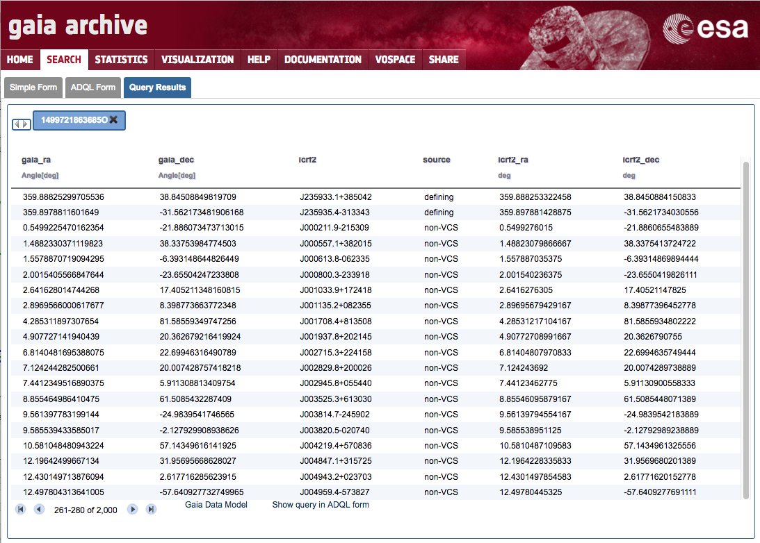
-
Gaia to ICRF2 positional differences computation
The position difference between Gaia and ICRF2 can also be computed within the archive adding two new columns to the output: ra_diff and dec_diff (units: mas)
SELECT gaia.ra AS gaia_ra, gaia.dec AS gaia_dec, icrf2.icrf2, icrf2.source, icrf2.raj2000 AS icrf2_ra, icrf2.dej2000 AS icrf2_dec, (gaia.ra - icrf2.raj2000) * cos(radians(icrf2.dej2000)) * 3600000 AS ra_diff, (gaia.dec - icrf2.dej2000) * 3600000 AS dec_diff FROM gaiadr1.aux_qso_icrf2_match AS gaia JOIN user_<username>.icrf2 AS icrf2 ON gaia.icrf2_match = icrf2.icrf2 -
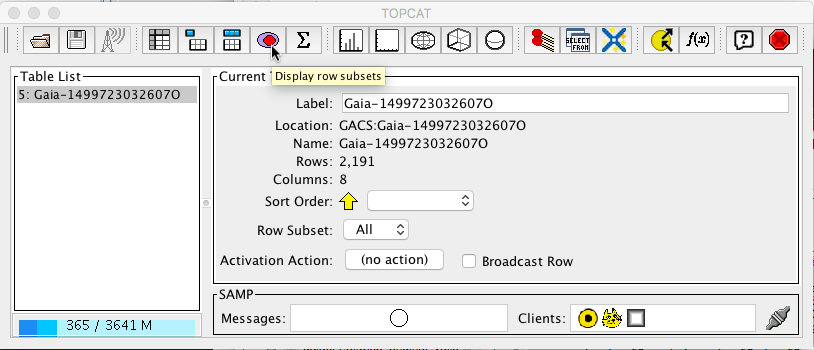
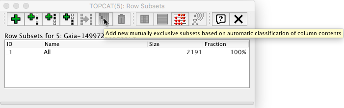
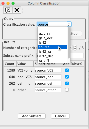
Data export to Topcat and representation
The table can be exported to the Topcat visualization tool via SAMP following ‘White dwarfs tutorial’ steps 15-17. The data will be divided into three subsets according to the contents of column 'source'
We will now represent dec_diff vs ra_dif as a 2D plot
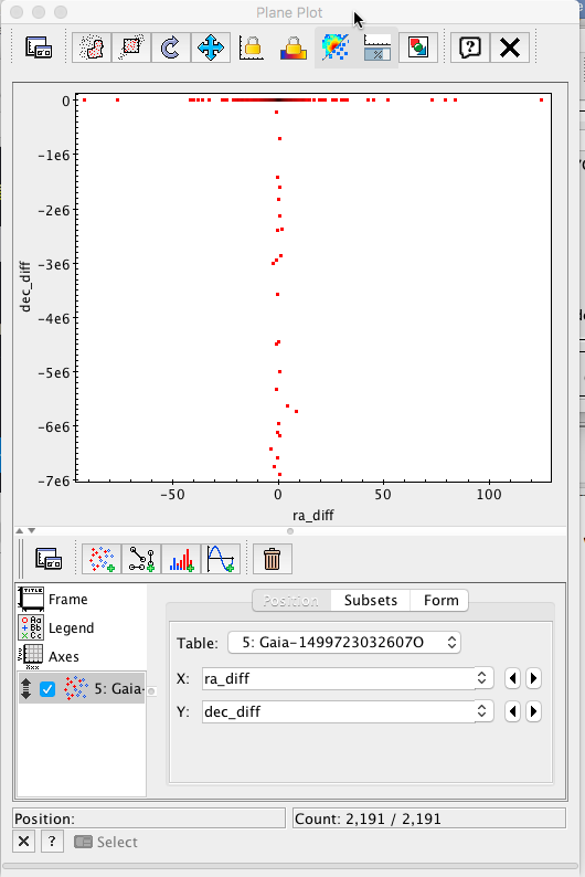
Initially, only the points presenting big discrepancies are apparent. Changing the plot range to ±10 mas in both axes, a much more informative plot is obtained.
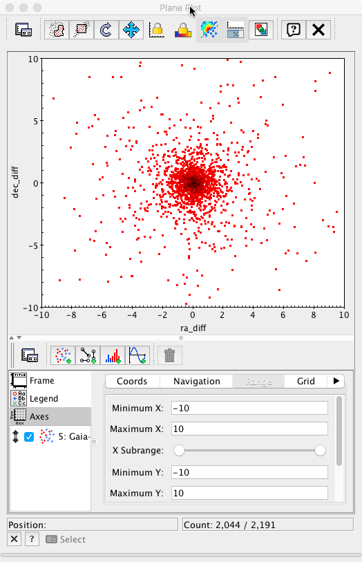
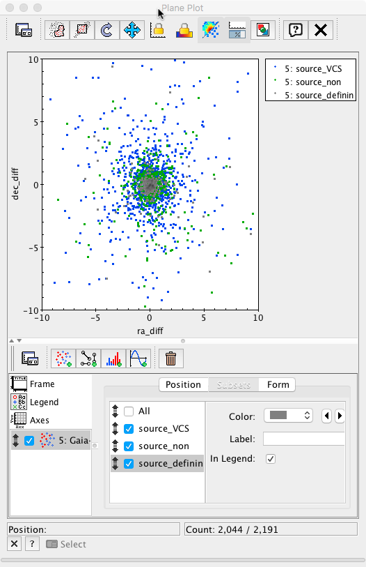
Finally, each subset can be plotted using different colours to reveal the behaviour of the different subsamples. This plot is equivalent to Fig.7 top right panel in Mignard et al. 2016.
-
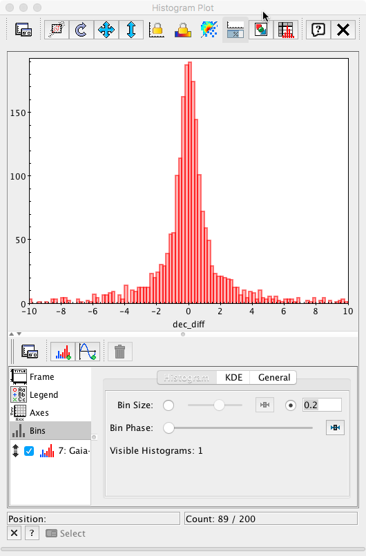
Gaia to ICRF2 positional differences histogram
The 2D data studied in the previous sections can also be displayed as a collection of 1D histograms. This can directly be carried out within most plotting programs, such as Topcat. However, this approach might become impractical when the number of data points reach billions in size (far from the case for ICRF sources). The following query shows how to compute a histogram directly within the Archive:
SELECT 0.2 * index AS dec_diff, n from ( SELECT floor(5 * (gaia.dec - icrf2.dej2000) * 3600000 + 0.1) AS index, count(*) AS n FROM gaiadr1.aux_qso_icrf2_match AS gaia JOIN user_<username>.icrf2 AS icrf2 ON gaia.icrf2_match = icrf2.icrf2 GROUP BY index ) AS subquery ORDER BY dec_diffwhere an intermediate integral index is defined such that the difference in declination is 0.2 mas for each increment of a full init. The accumulations are carried out in a subquery. The outer query reverses the multiplying factor to recover the original mas scale. The output data can then be exported to Topcat and represented as a 1D histogram, using the weighting the 'dec_diff' column as a function of the 'n' number of objects in that bin.
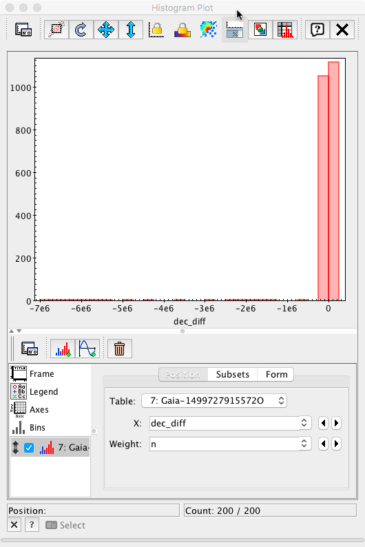
After adjusting the x-axis range to ±10 mas
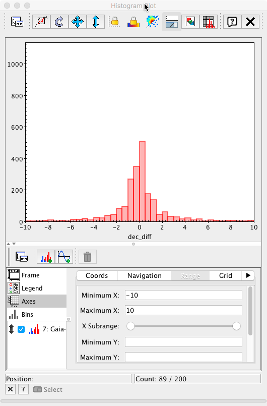
and the bin size to 0.2 mas (the value used in the Archive query), the plot is now equivalent to Fig. 6 left panel in Mignard et al. 2016.


- Removed a total of (8) style text-align:center;
- Removed a total of (25) style text-align:justify;
- Removed a total of (1) style font-weight:normal;
- Removed a total of (1) style margin:0;
- Removed a total of (1) align=left.
Cluster Analysis GUI
Authors: Raúl Gutiérrez, Alcione Mora, José Hernández
This is a tutorial is focused on possible scientific exploration exercise using the Gaia Archive. Realistic science use cases created from users are really welcome and they could be shared in this section with the proper reference/contact point.
We are going to explore a known cluster as the Pleiades (m45) using Gaia data. First, we are going to retrieve all the available data in the region of interest:
-
As we are going to use the private storage area, we have to log in the archive.
-
Go to Search → Simple Form. In positional search, enter "pleiades" in the field "Name". Once it is resolved, select a 2 degrees search radius and make sure "Gaia source" is selected. Click on "Show Query" button.
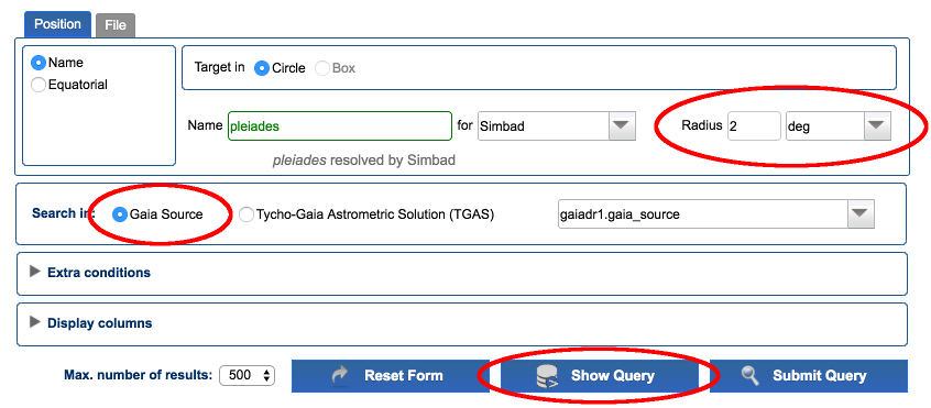
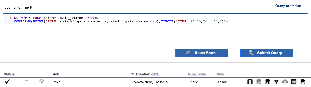
-
Enter "m45" in the field
Job name. Edit the ADQL query and remove theTOP 500restriction. The query should be:SELECT * FROM gaiadr1.gaia_source WHERE CONTAINS(POINT(gaiadr1.gaia_source.ra,gaiadr1.gaia_source.dec),CIRCLE(56.75,24.1167,2))=1Execute the query. Around 1e5 results are found.
-
The number of results are small enough to be represented by a local application. Open Topcat and click
Send to SAMPbutton. As the job is private, Topcat will ask for your credentials.
Once the data have been loaded, you could show the results in the sphere, or create a proper motion plot to identify the cluster.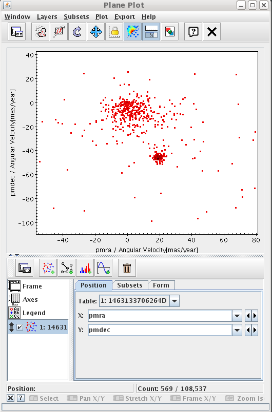
-
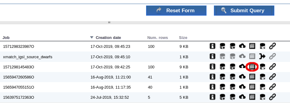
Go to the archive and filter data by quality. For that, create a new DB table in your local environment from the job results clicking on the corresponding upload icon (see image):

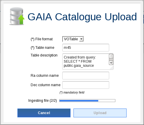

Enter "m45PmFilter" as job name and perform the next query (do not forget to replace <username> with your user name):
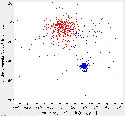
SELECT * FROM user_<username>.m45 WHERE abs(pmra_error/pmra)<0.10 AND abs(pmdec_error/pmdec)<0.10 AND pmra IS NOT NULL AND abs(pmra)>0 AND pmdec IS NOT NULL AND abs(pmdec)>0;Execute the query. You can send the results to Topcat via SAMP and plot the new results over the proper motion plot to see the sources with sufficient proper motion quality.
-
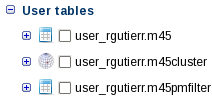
Create the table
m45pmfilterfromm45PmFilterjob results. Now we are going to take the candidate objects to be in the cluster. Based on the proper motion plot, we execute the next filter:SELECT * FROM user_<username>.m45pmfilter WHERE pmra BETWEEN 15 AND 25 AND pmdec BETWEEN -55 AND -40;Name the job as
m45clusterand execute the job. You could send the results to Topcat and plot over the previous proper motion plots.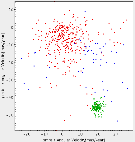
-
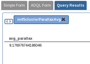
Using the ADQL interface we can perform analysis queries on the results. Create the table
m45clusterfromm45clusterjob results. Name the job asm45clusterParallaxAvg. Execute the next query:SELECT avg(parallax) as avg_parallax FROM user_<username>.m45clusterExecute the query and show the results using the corresponding button from the job results.
-
Now, we want to add information from other catalogues. To do so, we will make use of the crossmatch functionality of the archive. We need to identify which columns of our table have the geometrical information (
raanddecin our case). Selectm45clustertable by checking its check box and click on theEdit tablebutton. Find columnraand set the flagRa. Find the columndecand set the flagDec. Click onUpdate button.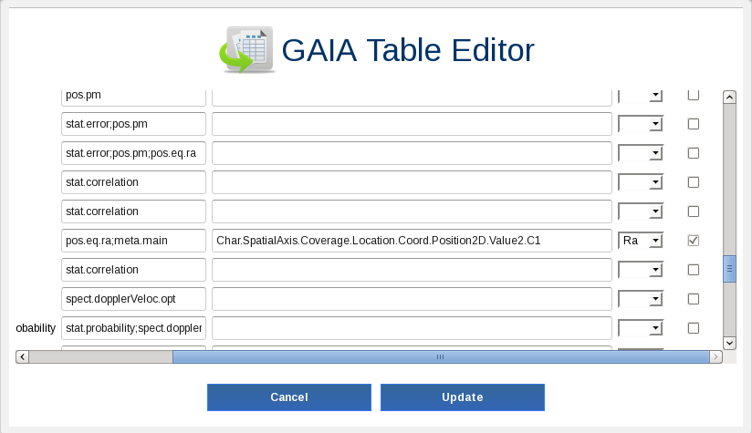
This action will create a positional index on Ra and Dec, and the table will be identified as a geometrical table. This allows the use of the crossmatch functionality.
-
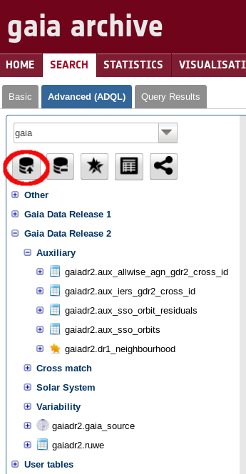
Click on
crossmatchbutton. Selectuser_<username>.m45clusterforTableAandgaiadr1.twomass_original_validforTableB. Click onExecute.
This will create a new job of crossmatch type and a new table calledxmatch_m45cluster_tmass_original_valid. This table is a joint table betweenm45clusterandtwomass_original_validtables. A helper function is available in the crossmatch job to create a join query between the two tables. -
To create a table with all the information from the two tables, click in the
Show join querybutton of the crossmatch job. A query like this is automatically loaded in the ADQL query panel:SELECT c."dist", a."dec", a."m45cluster_oid", a."ra", a."astrometric_chi2_ac", a."astrometric_chi2_al", a."astrometric_delta_q", a."astrometric_excess_noise", a."astrometric_excess_noise_sig", a."astrometric_go_f", a."astrometric_n_obs_ac", a."astrometric_n_obs_al", a."astrometric_n_outliers_ac", a."astrometric_n_outliers_al", a."astrometric_params_solved", a."astrometric_primary_flag", a."astrometric_priors_used", a."astrometric_rank_defect", a."astrometric_relegation_factor", a."astrometric_weight_ac", a."astrometric_weight_al", a."dec_error", a."dec_parallax_corr", a."dec_pmdec_corr", a."dec_pmra_corr", a."dec_pmradial_corr", a."m45_oid", a."m45pmfilter_oid", a."matched_observations", a."parallax", a."parallax_error", a."parallax_pmdec_corr", a."parallax_pmra_corr", a."parallax_pmradial_corr", a."phot_bp_mean_flux", a."phot_bp_mean_flux_error", a."phot_bp_mean_mag", a."phot_bp_n_obs", a."phot_g_mean_flux", a."phot_g_mean_flux_error", a."phot_g_mean_mag", a."phot_g_n_obs", a."phot_rp_mean_flux", a."phot_rp_mean_flux_error", a."phot_rp_mean_mag", a."phot_rp_n_obs", a."phot_variable_flag", a."pmdec", a."pmdec_error", a."pmdec_pmradial_corr", a."pmra", a."pmradial", a."pmradial_error", a."pmra_error", a."pmra_pmdec_corr", a."pmra_pmradial_corr", a."ra_dec_corr", a."radial_velocity", a."radial_velocity_constancy_probability", a."radial_velocity_error", a."ra_error", a."random_index", a."ra_parallax_corr", a."ra_pmdec_corr", a."ra_pmra_corr", a."ra_pmradial_corr", a."ref_epoch", a."scan_direction_mean_k1", a."scan_direction_mean_k2", a."scan_direction_mean_k3", a."scan_direction_mean_k4", a."scan_direction_strength_k1", a."scan_direction_strength_k2", a."scan_direction_strength_k3", a."scan_direction_strength_k4", a."solution_id", a."source_id", b."dec", b."ra", b."designation", b."err_ang", b."err_maj", b."err_min", b."ext_key", b."h_m", b."h_msigcom", b."j_date", b."j_m", b."j_msigcom", b."k_m", b."k_msigcom", b."ph_qual", b."tmass_oid" FROM user_<username>.m45cluster AS a, public.tmass_original_valid AS b, user_<username>.xmatch_m45cluster_tmass_original_valid AS c WHERE (c.m45cluster_m45cluster_oid = a.m45cluster_oid AND c.tmass_original_valid_tmass_oid = b.tmass_oid)Name the job as
xmatchand execute it. Show the results and verify that both Gaia and 2Mass data are present. -
Now, we are going to use the sharing functionality of the archive to share this results with some colleagues. First, create a new table
cluster_2massfrom the previous job. Go to the tabSHARE > Groupsand create a group calledcluster. The new group appears in the tree. Select the group and click onEdit. Use theUser to includefield to search for your colleague click on add. Repeat this search to add any other colleagues you want. Then click onUpdate. The group has been updated with the new members.
Return to the ADQL search page, check thecluster_2masstable and click onSharebutton. Select groupcluster, clickAddand thenUpdate. You will see that a littleShareicon is added to the table icon. From this moment, the users inclustergroup will be notified and they will have access to this table.


- Removed a total of (10) style text-align:center;
- Removed a total of (18) style text-align:justify;
- Removed a total of (1) style font-weight:normal;
- Removed a total of (19) style margin:0;
- Removed a total of (1) align=left.
- Removed a total of (10) style display:block;
Cluster Analysis Python
Authors: Deborah Baines
This tutorial has taken the Cluster analysis tutorial and adapted it to python. The tutorial uses the Gaia TAP+ (astroquery.gaia) module .
This tutorial is focused on a possible scientific exploration exercise for a known cluster, the Pleiades (M45), using data from the Gaia Archive.
You can import and run this tutorial in your own Jupyter Notebook using this file: Download
First, we import all the required python modules:
import astropy.units as u
from astropy.coordinates.sky_coordinate import SkyCoord
from astropy.units import Quantity
from astroquery.gaia import Gaia
%matplotlib inlineimport matplotlib.pyplot as plt
import numpy as np
# Suppress warnings. Comment this out if you wish to see the warning messages
import warnings
warnings.filterwarnings('ignore')
from astroquery.gaia import Gaia
tables = Gaia.load_tables(only_names=True)
for table in (tables):
print (table.get_qualified_name())
query = "SELECT * FROM gaiadr1.gaia_source WHERE DISTANCE(ra,dec,56.75,24.1167) <2"
job   = Gaia.launch_job_async(query, dump_to_file=True)
print (job)
r = job.get_results()
print (r['source_id'])
plt.scatter(r['pmra'], r['pmdec'], color='r', alpha=0.3)
plt.xlim(-60,80)
plt.ylim(-120,30)
plt.show()

query = "SELECT * FROM gaiadr1.gaia_source \
WHERE DISTANCE(ra,dec,56.75,24.1167) <2 \
AND abs(pmra_error/pmra)<0.10 AND abs(pmdec_error/pmdec)<0.10 \
AND pmra IS NOT NULL AND abs(pmra)>0 \
AND pmdec IS NOT NULL AND abs(pmdec)>0"

job2 = Gaia.launch_job_async(query, dump_to_file=True)
j = job2.get_results()
print (j['source_id'])
plt.scatter(r['pmra'], r['pmdec'], color='r', alpha=0.3)
plt.scatter(j['pmra'], j['pmdec'], color='b', alpha=0.3)
plt.xlim(-60,80)
plt.ylim(-120,30)
plt.show()

query = "SELECT * FROM gaiadr1.gaia_source \
WHERE DISTANCE(ra,dec),56.75,24.1167) <2 \
AND abs(pmra_error/pmra)<0.10 AND abs(pmdec_error/pmdec)<0.10 \
AND pmra IS NOT NULL AND abs(pmra)>0 AND pmdec IS NOT NULL \
AND abs(pmdec)>0 AND pmra BETWEEN 15 AND 25 AND pmdec BETWEEN -55 AND -40"

job3  = Gaia.launch_job_async(query, dump_to_file=True)
m45cluster = job3.get_results()
print (m45cluster['parallax'])
plt.scatter(r['pmra'], r['pmdec'], color='r', alpha=0.3)
plt.scatter(j['pmra'], j['pmdec'], color='b', alpha=0.3)
plt.scatter(m45cluster['pmra'], m45cluster['pmdec'], color='g', alpha=0.3)
plt.xlim(-60,80)
plt.ylim(-120,30)
plt.show()

avg_parallax = np.mean(m45cluster['parallax'])
stddev_parallax = np.std(m45cluster['parallax'])
print (avg_parallax, stddev_parallax)
job4 = Gaia.launch_job_async(
"SELECT * FROM gaiadr1.gaia_source AS g, \
gaiadr1.tmass_best_neighbour AS tbest, gaiadr1.tmass_original_valid AS tmass \
WHERE g.source_id = tbest.source_id AND tbest.tmass_oid = tmass.tmass_oid \
AND CONTAINS(POINT(g.ra,g.dec),CIRCLE(56.75,24.1167,2))=1 \
AND abs(pmra_error/pmra)<0.10 \
AND abs(pmdec_error/pmdec)<0.10 \
AND pmra IS NOT NULL AND abs(pmra)>0 \
AND pmdec IS NOT NULL AND abs(pmdec)>0 \
AND pmra BETWEEN 15 AND 25 \
AND pmdec BETWEEN -55 AND -40", dump_to_file=False)
p = job4.get_results()
print (p['phot_g_mean_mag', 'j_m', 'h_m', 'ks_m'])
job5 = Gaia.launch_job_async(
"SELECT * FROM gaiadr1.gaia_source \
INNER JOIN gaiadr1.tmass_best_neighbour
  ON gaiadr1.gaia_source.source_id = gaiadr1.tmass_best_neighbour.source_id \
INNER JOIN gaiadr1.tmass_original_valid
  ON gaiadr1.tmass_original_valid.tmass_oid = gaiadr1.tmass_best_neighbour.tmass_oid \
WHERE DISTANCE(ra,dec,56.75,24.1167) <2 \
AND abs(pmra_error/pmra)<0.10 \
AND abs(pmdec_error/pmdec)<0.10 \
AND pmra IS NOT NULL AND abs(pmra)>0 \
AND pmdec IS NOT NULL AND abs(pmdec)>0 \
AND pmra BETWEEN 15 AND 25 \
AND pmdec BETWEEN -55 AND -40", dump_to_file=True)
test = job5.get_results()
print (test['phot_g_mean_mag', 'j_m', 'h_m', 'ks_m'])
plt.scatter(r['pmra'], r['pmdec'], color='r', alpha=0.3)
plt.scatter(j['pmra'], j['pmdec'], color='b', alpha=0.3)
plt.scatter(m45cluster['pmra'], m45cluster['pmdec'], color='g', alpha=0.3)
plt.scatter(test['pmra'], test['pmdec'], color='y', alpha=0.3)
plt.xlim(-60,80)
plt.ylim(-120,30)
plt.show()

- Removed a total of (34) style text-align:left;
- Removed a total of (52) style text-align:right;
- Removed a total of (1) style font-weight:normal;
- Removed a total of (71) style font-weight:bold;
- Removed a total of (20) style font-style:italic;
- Removed a total of (53) style border:none;
- Removed a total of (52) style overflow:auto;
- Removed a total of (136) style margin:0;
- Removed a total of (66) style padding:0;
- Removed a total of (1) align=left.
- Removed a total of (31) style display:block;
White Dwarfs Exploration
Authors: Jesús Salgado, Juan-Carlos Segovia
This is a tutorial is focused on possible scientific exploration exercise using the Gaia Archive. Realistic science use cases created from users are really welcome and they could be shared in this section with the proper reference/contact point.
We are going to explore white dwarfs observed by Gaia. First, we have a typical known white dwarfs catalogue at Vizier:
-
Go to Vizier to:
IR photometry of 2MASS/Spitzer white dwarfs
http://vizier.u-strasbg.fr/viz-bin/VizieR-3?-source=J/ApJ/657/1013&-out.max=50&-out.form=HTML%20Table&-out.add=_r&-out.add=_RAJ,_DEJ&-sort=_r&-oc.form=sexa - Download the catalogue by:
- Select in Preferences:
max=unlimited, output format = VOTable. - Click on Submit.
- A file called
vizier_votable.votwill be created.
- Select in Preferences:
-
Open in a different tab the Gaia Archive:
https://archives.esac.esa.int/gaia/ -
Log in Gaia Archive.
-
Click on SEARCH Tab and, inside it, the Advanced ADQL Form.
-
Click on the upload table button
and select the
vizier_votable.votVOTable. -
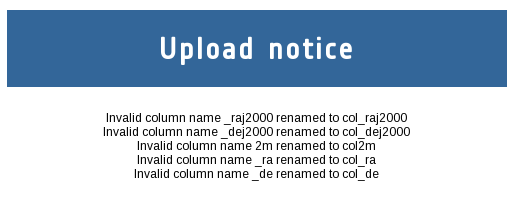
Use as table name "dwarfs" and click on the Upload button. As some of the column names of the downloaded VOTable are not compatible with TAP/ADQL, the system will automatically rename them showing the next notice:
-
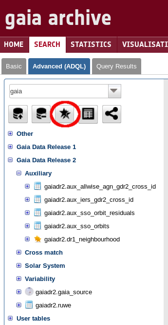
Select the uploaded table
user_<your_login_name>.dwarfs(under 'User tables') and click on the edit table button: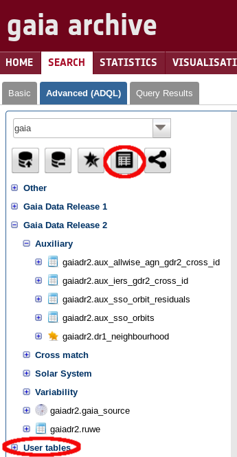
-
For column
col_raj2000select the flagRa. And for columncol_dej2000select the flagDec. Then clickUPDATE. The table icon in the tree will change to a "Positional indexed table"
-
Inspect the table content inside Gaia Archive. Type in the form at the top of the page:
select top 100 * from user_<your_user_name>.dwarfswhere <your_user_name> is your own username, and click 'Submit Query'. A new job will start to be exectued and, when finished, the table result could be inspected by clicking on the "Display top 2000 results" button:
Now, we want to obtain metadata of Gaia catalogues for these sources. In order to do that, counterparts should be found by the execution of a crossmatch operation. A positional crossmatch (identification by position) will be executed. More complex algorithms will be offered in future Gaia Archive versions.
-
Click on the crossmatch button:
-
Select as Table A:
public.igsl_sourceand as Table B:user_<your_user_name>.dwarfswith a radius of 1 arcsecondNote: IGSL is a combination catalogue from other external catalogues. It has the size of the expected future Gaia catalogue and a synthetic photometry on band G (Gaia). The calculation of this photomtetry could fail for peculiar objects. See more info on IGSL at: http://www.cosmos.esa.int/web/gaia/iow_20131008
-
Execute the crossmatch. A new job will start. At the end of the execution, a new join table (called
xmatch_igsl_source_dwarfsby default) will be created between IGSL and "dwarfs" catalogues. -
When finished, click on the "Show join query"
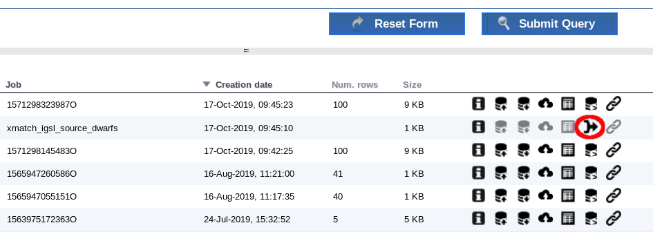
This query is an example on how to contain all the metadata of the two catalogues. Reduce the content of the metadata by replacing the
SELECTpart of the ADQL sentence as followsSELECT a."source_id", b."dwarfs_oid", b."name", a."ra", a."dec", b."col_raj2000", b."col_dej2000", a."mag_g", b."f_hmagc", b."f_jmagc", b."f_kmagc", b."hmag2", b."hmagc", b."jmag2", b."jmagc", b."kmagc", b."ksmag2"Note: FROM and WHERE conditions must be preserved
This query will contain the ids of the source in both catalogues (to explore possible duplications), the name of the dwarf stars and magnitudes from both catalogues.Click on "Submit Query" to launch a new job.
-
Open the VO application Topcat:
http://www.star.bris.ac.uk/~mbt/topcat/topcat-lite.jnlp -
Download results and open them in Topcat.
Click on Download button
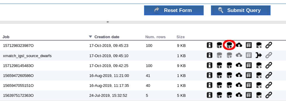
Open results with Topcat.
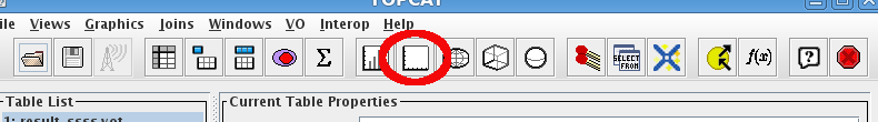
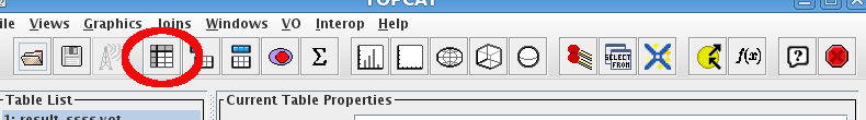
-
on the "Plane Plotting Window" button
-
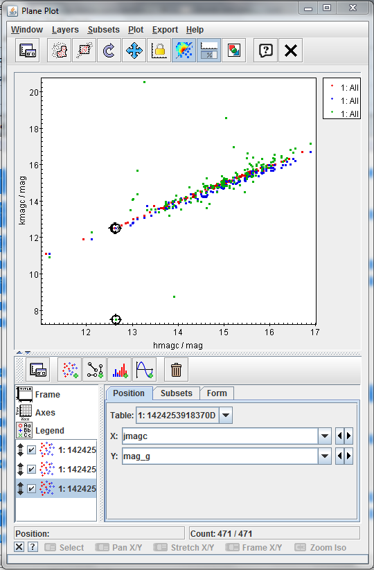
Add, by clicking on the "Add a new positional control to the stack", to create three plots:
- hmagc versus kmagc
- jmagc versus kmagc
- jmagc versus mag_g
The result should be as follows
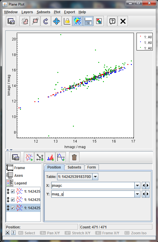
Most of the points are located in a clear line except some few up and two of them clearly below it. That could imply that they emits on the G band more than the expected (as the G band is synthetic for IGSL, this is not fully clear) or that the crossmatch is not fully correct for these sources.
Click on the "Display table cell data" button on the main Topcat window.
-
Click on the Plan Plot, one at once, on the two strange sources. Once you click on one source, the two plots will be synchronized
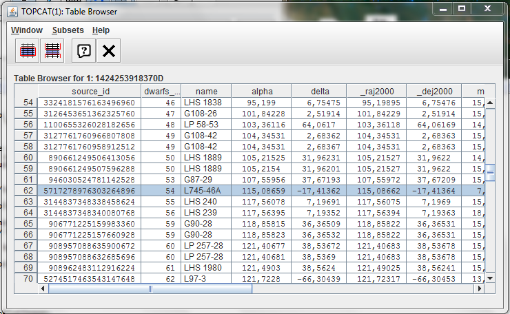
-
Checking the name column in the Table browser, the two sources are:
- LTT 4816
- L745-46A
The first object has been identified as a pulsating white dwarf and the second as a simple white dwarf.
The analysis of the result could suggest a failure on the calculation of the synthetic G magnitude for these objects or some peculiarity on the emission.


- Removed a total of (13) style text-align:center;
- Removed a total of (1) style font-weight:normal;
- Removed a total of (1) style margin:0;
- Removed a total of (1) align=left.
Variable sources (DR1)
Author: Alcione Mora
![]()
Gaia DR1 contains information on a selection of pulsating variables, mostly in the Large Magellanic Cloud, in addition to the other deliverables, mainly the gaia_source table, which contains the astrometry and average photometry for 1.14 billion sources in the sky.
This is an intermediate level tutorial that assumes a basic knowledge of the general interface and workflow. The introductory tutorials White dwarfs exploration and Cluster analysis are recommended in case of difficulties following this exercise.
Variable sources
The main references dealing with the analysis of variable star light curves in DR1 are Eyer et al. 2017 and Clementini et al. 2016 A&A 595A, 133C. The former provides an overview of the all the variability analyses carried out, while the latter focuses on the Cepheids and RR Lyrae pipeline and the results finally published in DR1. The Clementini et al. 2017 abstract is reproduced below.
Context. The European Space Agency spacecraft Gaia is expected to observe about 10,000 Galactic Cepheids and over 100,000 Milky Way RR Lyrae stars (a large fraction of which will be new discoveries), during the five-year nominal lifetime spent scanning the whole sky to a faint limit of G = 20.7 mag, sampling their light variation on average about 70 times.
Aims. We present an overview of the Specific Objects Study (SOS) pipeline developed within the Coordination Unit 7 (CU7) of the Data Processing and Analysis Consortium (DPAC), the coordination unit charged with the processing and analysis of variable sources observed by Gaia, to validate and fully characterise Cepheids and RR Lyrae stars observed by the spacecraft. The algorithms developed to classify and extract information such as the pulsation period, mode of pulsation, mean magnitude, peak-to-peak amplitude of the light variation, subclassification in type, multiplicity, secondary periodicities, and light curve Fourier decomposition parameters, as well as physical parameters such as mass, metallicity, reddening, and age (for classical Cepheids) are briefly described.
Methods. The full chain of the CU7 pipeline was run on the time series photometry collected by Gaia during 28 days of ecliptic pole scanning law (EPSL) and over a year of nominal scanning law (NSL), starting from the general Variability Detection, general Characterization, proceeding through the global Classification and ending with the detailed checks and typecasting of the SOS for Cepheids and RR Lyrae stars (SOS Cep&RRL). We describe in more detail how the SOS Cep&RRL pipeline was specifically tailored to analyse Gaia's G-band photometric time series with a south ecliptic pole (SEP) footprint, which covers an external region of the Large Magellanic Cloud (LMC), and to produce results for confirmed RR Lyrae stars and Cepheids to be published in Gaia Data Release 1 (Gaia DR1).
Results. G-band time series photometry and characterisation by the SOS Cep&RRL pipeline (mean magnitude and pulsation characteristics) are published in Gaia DR1 for a total sample of 3194 variable stars (599 Cepheids and 2595 RR Lyrae stars), of which 386 (43 Cepheids and 343 RR Lyrae stars) are new discoveries by Gaia. All 3194 stars are distributed over an area extending 38 degrees on either side from a point offset from the centre of the LMC by about 3 degrees to the north and 4 degrees to the east. The vast majority are located within the LMC. The published sample also includes a few bright RR Lyrae stars that trace the outer halo of the Milky Way in front of the LMC.
Gaia Archive tables
The variability data are distributed among the following tables:
- variable_summary. It contains a list of the stars classified in gaia_source as variables, together with the first fundamental frequency and best classification.
- cepheid. Additional fit parameters for Cepheids, including best sub-class and light curve Fourier analysis (period, peak-to-peak amplitude, first to second harmonic ratio, ...)
- rrlyrae. Similar results, but for RR Lyrae.
- phot_variable_time_series_gfov. The G-band light curves: fluxes, errors and magnitudes as a function of time.
- phot_variable_time_series_gfov_statistical_parameters. Basic statistical analysis of each light curve: number of points, first fourth moments, minimum, maximum, median, ...
In addition, gaia_source has the specific field phot_variable_flag set to 'VARIABLE' for all variable stars in this data release.
Getting summary data
The following queries show how to retrieve a basic summary of the first 10 Cepheids and RR Lyrae in the archive. Note the contents of four different tables is joined to provide a full overview.
Cepheids
SELECT TOP 10 gaia.source_id, gaia.ra, gaia.dec, gaia.parallax, variable.classification, variable.phot_variable_fundam_freq1, phot_stats.mean, cepheid.peak_to_peak_g, cepheid.num_harmonics_for_p1, cepheid.r21_g, cepheid.phi21_g, cepheid.type_best_classification, cepheid.type2_best_sub_classification, cepheid.mode_best_classification FROM gaiadr1.gaia_source AS gaia INNER JOIN gaiadr1.variable_summary AS variable ON gaia.source_id = variable.source_id INNER JOIN gaiadr1.phot_variable_time_series_gfov_statistical_parameters AS phot_stats ON gaia.source_id = phot_stats.source_id INNER JOIN gaiadr1.cepheid AS cepheid ON gaia.source_id = cepheid.source_id
RR Lyrae
SELECT TOP 10 gaia.source_id, gaia.ra, gaia.dec, gaia.parallax, variable.classification, variable.phot_variable_fundam_freq1, phot_stats.mean, rrlyrae.peak_to_peak_g, rrlyrae.num_harmonics_for_p1, rrlyrae.r21_g, rrlyrae.phi21_g, rrlyrae.best_classification FROM gaiadr1.gaia_source AS gaia INNER JOIN gaiadr1.variable_summary AS variable ON gaia.source_id = variable.source_id INNER JOIN gaiadr1.phot_variable_time_series_gfov_statistical_parameters AS phot_stats ON gaia.source_id = phot_stats.source_id INNER JOIN gaiadr1.rrlyrae AS rrlyrae ON gaia.source_id = rrlyrae.source_id
The results for the RR Lyrae query are summarised below:


Light curve reconstruction and folding
G-band light curves are only provided for objects classified as variable stars in DR1. They are included in table phot_variable_time_series_gfov. It contains one row per star and observing time. The main fields are:
- source_id. The source identifier.
- observation_time. The time scale is TCB, measured in Julian days. The zero point is 2010-01-01T00:00:00.
- g_flux, g_error. Units are electrons per second.
- g_magnitude. Vega scale. Converted from g_flux using the zero points in table ext_phot_zero_point.
- rejected_by_variability_processing. Identified outliers.
Magnitude errors are not provided, because they cannot be easily quantified with a single number for low signal to noise fluxes. In the high signal regime, the following approximate relation can be used.
ΔG ≈ 2.5/log(10) * Δf/f
where G is the magnitude and f the flux. Note that using fluxes instead of magnitudes is recommended whenever precise analyses are required (e.g. photometric system cross-calibration, spectral energy distribution construction, ...).
The following query illustrates how to retrieve the light curve in magnitudes of a given variable: the RR Lyrae with source_id = 5284240582308398080 in this example.
SELECT curves.observation_time, mod(curves.observation_time - rrlyrae.epoch_g, rrlyrae.p1)/ rrlyrae.p1 as phase, curves.g_magnitude, 2.5/log(10)* curves.g_flux_error/ curves.g_flux AS g_magnitude_error, rejected_by_variability_processing AS rejected FROM gaiadr1.phot_variable_time_series_gfov AS curves INNER JOIN gaiadr1.rrlyrae AS rrlyrae ON rrlyrae.source_id = curves.source_id WHERE rrlyrae.source_id = 5284240582308398080
The output contains the time (TCB), phase, G-band magnitude and estimated error and a flag indicating whether this point has been used by the variability processing. The phase is estimated folding the time using the best fit period. The origin is taken at the epoch of maximum flux in the fitted harmonic model.
The data can then be exported for further use. Topcat plots of the unfolded and folded light curves with error bars are provided below.

Miscellaneous plots from Clementini et al. 2016
Additional ADQL queries are provided to reproduce some plots (using Topcat) originally included in the Clementini et al. (2016)
Fig. 28. Histogram of RR Lyrae periods (all Gaia sources)
SELECT floor(p1 * 50) / 50 AS period, count(*) AS n FROM gaiadr1.rrlyrae GROUP BY period ORDER BY period

Fig. 30 top panel. RR Lyrae period – G-band amplitude diagram
SELECT p1, peak_to_peak_g, best_classification FROM gaiadr1.rrlyrae
Two exclusive subsets are created based on the best_classification column.

Fig. 34 top panel. Cepheids period-luminosity diagram
SELECT p1, int_average_g, type_best_classification, type2_best_sub_classification, mode_best_classification FROM gaiadr1.cepheid

Topcat views of the query result shown as a table and the corresponding subset definition used in the plot above are included below.


- Removed a total of (15) style text-align:center;
- Removed a total of (42) style text-align:justify;
- Removed a total of (11) style font-weight:normal;
- Removed a total of (1) style margin:0;
- Removed a total of (1) align=left.