Gaia Archive Visualisation Service (GAVS)

Authors: André Moitinho

Overview

The Gaia Archive Visualisation Service (GAVS) provides an interactive visual exploration environment for the Gaia ESA Archive.

The size and information content of Gaia archive, with almost two billion stars, can be overwhelming. GAVS is designed for helping to make this information intelligible.

This is achieved by using tricks like smart indexing of the data and pre-computing views for offering detail on demand. Because specific pre-computations for each visualisation are necessary, not all possible views and transformations of Gaia data can be offered. Instead, GAVS offers visual tools that help querying and extracting smaller subsets from the Gaia archive which can be downloaded and explored with other advanced software.

GAVS provides a multi-panel visualisation desktop in a browser tab. The panels are resizeable, moveable and their plots can be panned and zoomed. The figure below illustrates how a working setup might look.

Currently, GAVS provides several visual representations of Gaia's Data Release 3 (Gaia DR3) as 1D histograms, 2D scatter plots and binned plots, 3D scatter plots as well as all-sky source density and integrated luminosity maps.

General Functions

​​​​

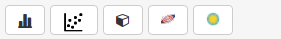
• Add new plot: the menu bar on the upper left of the browser tab offers a variety of visualisations in several initial sizes and aspect ratios. From left to right: 1D histograms, 2D scatter and binned plots, 3D scatter plots, HiPS maps, FITS images.
  
• Move window: drag window bar
• Resize window: drag lower right corner
• Close window: click "X" button on right of the window bar
• Pan: drag plot area
• Zoom: +/- buttons on right of plot area will zoom in/out with respect to the center of the plot. Mouse scroll will zoom in/out around the position of the mouse.
• Reset view: click on "+" cross on the right side of the window bar
• Presets and configurations: a pop-up menu will appear by clicking the sprocket-wheel button on the left of the window bar. Options depend on the kind of plot and are described further below.
• Save hard copy: the window bar of 1D, 2D, and 3D panels include a button for downloading print quality snapshots in PNG format (icon on the right of this line). Hard copies in the Aladin and JS9 plug-ins can be created using the interfaces provided by those applications.
• Annotation tools: a basic toolbox for drawing shapes and text is provided for annotating

In addition, depending on the plot type other functionalities are available. These include linked views capabilities, the looking glass and regions buttons seen in some window bars. They are described below.

Linked views

Linked views can be seen in action in the overview figure above. A maker signals the same star in 3 different scatter plots and highlights the bin to which it belongs in a histogram.

Gaia data are highly multidimensional. However, the number of dimensions that a plot can represent well is normally small. This limits exploration of the data set. One way around this problem is to have linked views of panels showing different data attributes. Usually this means selecting a point in one plot (e.g. HR Diagram) and highlighting or marking it in another plot (e.g. proper motion diagram). This simple example shows how 4 attributes (dimensions) of data for a star (and its context) can be easily perceived.

In GAVS, clicking on a star will also draw a marker in the other plots in which the star is visible. Note that not all stars appear in all plots. As an example, there are much less stars with radial velocities (~33 million) than with positional or photometric data (over 1.5 billion). So a star in a plot based on radial velocities will in general exist in positional or photometric plots, but clicking on a positional or photometric plot will usually not place a marker on radial velocity based plot.

Linked views between scatter plots and histograms are also offered. Selecting a star in a scatter plot (2D) will highlight the bin which it belongs to in a histogram (1D). The converse feature, clicking on a bin highlighting the corresponding stars in a scatter plot, is planned for future releases of this service.

GAVS can display multiple visualisation layers in the same window. As an example, a 2D plot with three layers could be made of the positions of RR Lyrae in one colour, positions of all Gaia sources in another colour and a source count binned map in the background. Clicking will select sources from the uppermost (scatter plot) layer. The points and bins marked in the linked plots will also refer to their upper layer.

2D plots

Configurations

2D plots can be of two types: scatter plots and binned plots (e.g. 2D histogram). The figure above shows the configuration menus for scatter plots (left) and binned plots (right). Multiple layers of scatter and/or binned plots are supported.

The following text fields in both menus can be edited and will be updated in the plot in real time:

• Title. In this image it's the "Galactic Coordinates" at the top of the menu
• X label, Y Label. Changes labels in axes
• Names of Layers and Regions. The layer names used in the plot legend.

Regions can be made visible or invisible (tick checkbox) or deleted. More on Regions below in this guide.

Tips for scatter plots: The Form sub-menu allows changing the point shape, size, colour, as well as the background colour. Importantly, the colour picker provides a means to change the transparency of points. For large datasets, a good balance of size and transparency is important for producing useful visualisations. They should be changed according to the zoom level. As an example, for an overall view, one might want small points with some transparency. If the density contrast is very high, large points (for seeing isolated points) with higher transparency (for seeing structure in crowded regions) might be a good choice. For a very zoomed view, large points with no transparency could work best. GAVS provides an initial setup adequate for an overall view.

Tips for binned plots: Binned plots are arrays of pixels. In this version of GAVS, the value in each pixel is the number of sources that fall in it. In this case, the plot is in effect a 2D histogram. Future versions will allow setting the pixel values to statistics on other columns in the Gaia archive (e.g. integrated G flux).

Re-binning big data volumes like Gaia DR3 is a heavy operation and can take some minutes. However, GAVS caches the arrays, which means that those that are commonly requested (such as the defaults) will be shown quickly. The maximum number bins (pixels) in each axis is 1024. The default binned layer for a plot of Galactic coordinates (l, b) is 512x256 which is roughly 0.7x0.7 degrees/pixel close to the Galactic equator. To obtain high resolution maps, smaller areas must be used. The X and Y limits of the area are set under the "Axes" options. As an example, a higher resolution source count map of Ophiuchus can be obtained setting X between [-15, 5] and Y between [10, 20] and then adjusting the colour-map range. At 512x256 pixels, it has a resolution of roughly 2.3x2.3 arcmin/pixel. The image is shown below.

Tips for using layers: The upper layer is the most visible. The position of a layer can be changed by dragging the "+" symbol in its tab. Seeing layers below might require adding transparency to the points and to the background. In this version of GAVS only opaque colour maps are offered. This means that only one binned layer can be seen at a time and it should be below any other scatter plot layers.

The image below shows an example of a scatter plot with transparency over a binned plot with a black, blue and red colour map.

Looking glass

Centres the view port on a point of interest. Writing a position (coordinates separated by a space or a comma) will center the view port on that position. For spatial plots (galactic, equatorial and ecliptic coordinates), an object name can be given instead of coordinates. If the name can be resolved by the Sesame service at CDS, the view port will be centred on that position. Then just zoom in-out until the object of interest is seen.

Gaia archive and Simbad searches

Click to select a star. A second click (not double click) will make a pop-up will appear, like the one in the figure below.

In sky maps (galactic, equatorial and ecliptic coordinates) a pop-up interface offers a number of possibilities:

• Search the selected object in the Gaia ESA Archive. A query string for doing an ADQL search of the selected object in the Gaia Archive is produced. It can be copied and pasted in to the archive query interface.
• Search within a user defined radius (default is 10 arcmin) centred on the selected object. This will open a tab with the results of a SIMBAD query or produce an ADQL string for using in the Gaia Archive query interface.

Regions:

Regions is a feature supported by some astronomical image display software, most noticeably by the popular DS9 fits image viewer (and the JS9 web version, which is also a plug-in of GAVS). As stated in the DS9 regions web page, "Regions provide a means for marking particular areas of an image for further analysis. Regions may also be used for presentation purposes".

The next figure is a snapshot of the Regions menu and two created Regions.

Currently, GAVS only supports the creation of Polygons and Rectangles. Rectangles are created by clicking and dragging the mouse. Polygons are created by clicking on the positions of the vertices until the polygon is closed.

Regions can be modified with the "Edit Regions" options. Just move the small squares to change the shape. In the end, uncheck the  "Edit Regions" option.

Regions can be made visible and invisible, deleted and have their colours changed in the general 2D configurations panel.

Regions can be saved text files and loaded. This is useful for later reuse, sharing with other people and also for use with DS9/JS9. This last feature provides a degree of interoperability between GAVS and DS9/JS9. Saving joins all visible Regions. Regions can be excluded from the save by making them invisible in the Configuration menu.

NOTE: Region support is very limited at the moment. Regions created by GAVS can be read by DS9. However, regions created by DS9 can only be read by GAVS if Rectangles are written as polygons, coordinates must be in decimal degrees, either galactic or ICRS. In addition, GAVS cannot write, but can read DS9 "points", again in decimal galactic or ICRS degrees.

Point Regions can be handy for overlay of catalogues. The image below illustrates an overlay of the catalogue of open clusters by Dias et al. (2002, A&A, 389, 871 - Version 3.5, Jan 2016). The corresponding Regions file can be found here as an example. Region files for Milky Way globular clusters and nearby dwarf galaxies are also provided as examples.

Finally, one of the neat features in GAVS is that Regions can be used for generating ADQL queries for retrieving stars within an arbitrary polygon. It gives the user the power of visually creating simple ADQL queries in an easy way without having to know ADQL. The next figure illustrates this. Just click ADQL after creating the region. It will create a query string joining only the visible Regions.

1D plots

Currently, only histograms are supported. Histograms are computed in real time. This may take a few seconds, which is fast considering that some histograms represent the full Gaia DR3 with approximately 1.8 billion points. This real time computation gives a lot of flexibility to the histograms that can be produced. It is made possible by the data indexing scheme used in GAVS.

Configurations

The configuration menu provides several options for changing the look of a histogram.

The following text fields can be edited and will be updated in the plot in real time:

• Title. In this image it's the "Parallax" at the top of the menu
• X label, Y Label. Changes labels in axes
• Name of Layers. Layers can be made visible or invisible using the check box before their name. They can also be re-ordered by dragging the "+" symbol.

In addition the following options are offered:

• "nbins" scroll down for to specifying the number of bins or the bin size.
• "Total count" scroll down for to showing the histogram of total counts or highest bin normalised to 1
• limits for the X axis (limits in Y will be offered in the next version).

The remaining options are similar to those for the 2D scatter plot.
 

3D plots

GAVS offers a panel for 3D visualisation. This first experimental version is limited to displaying X,Y,Z positions in the sky, relative to the Sun. In this system, X increases towards the Galactic centre (the line of galactic longitude  l=0); Y increases towards the direction of Galactic rotation (l=90) and Z increases toward the north Galactic pole (the "up" direction in the default view). As with the 2D panel, detail is presented on demand. A progress bar in the upper right of the view port marks the loading of current level of detail. In this version, only stars with "good" parallaxes (better than 10%) are displayed.

Navigation is done with the mouse:

• rotate:  drag with left button clicked
• move in and out: mouse wheel or drag with middle button clicked
• move sideways: drag with right button clicked

Configurations

The configuration menu provides several options and tools for 3D.

The following text fields can be edited and will be updated in the plot in real time:

• Title. In this image it's the "parallax_over_error > 10" at the top of the menu
• X label, Y Label. Changes labels in axes
• Name of Layers. Only one layer is available in this version

In addition the following options are offered:

• 3D axes: draw 3D axes. Using the mouse wheel changes the space volume of the box.
• Crop to axes: only points within the box are visible. Note that the initial box is very small and no stars will be seen. Increasing the volume is required (mouse wheel to zoom out)
• Galactic coordinates: draw a sphere, centred on the Sun with Galactic coordinates marked.
• Minimap: show 2D projections of space with the camera position and pointing.
• Field of view: change field of view (units= degrees)
• Quality: change the maximum number of points shown in a given view. From low (less) to high (more). Higher increases the power consumption of the device used for connecting to GAVS.

The remaining options are similar to those for the 2D scatter plot.

 

Camera animation

The camera animation menu allows creating animations though different positions and orientations of the 3D camera (in other words, different views in the panel). This can be done by clicking "New path" in the camera animation menu.

A path is created by moving to a new location and orientation (mile markers), pressing the "+" button on the top right of the menu to mark the location, move again, "+"again, and so on. Names can be given to each mile marker in the "label field" . The mile markers can be edited by first clicking on the edit button on their left. Then un-tick "Edit path" in the camera animation menu and click play. An animation of the newly created path will be played in the 3D panel. 
The animations are specified as text files that can be saved to the user's computer (and then shared) and loaded with the save/load path options in the camera animation menu.

Disclaimer: The 3D panel is still in an experimental phase. It is not yet very robust and might hang or have non-intended behaviour.

Plug-ins

Besides the GAVS native plots, partial integration of external applications has been done. This allows building more extended exploration pipelines in a comprehensive environment.

The current version of GAVS includes:

• Aladin Lite: By default it displays a coloured integrated flux HiPS map produced with Gaia DR3 G, BP and RP fluxes. The "base image layer" menu item allows changing to a grayscale source count map or integrated flux maps in each of the Gaia photometric bands.
• JS9: By default it displays a density fits map produced with Gaia DR1 data. JS9 can be used for displaying user fits images (e.g. from other observations) making it possible to explore them in the context of the Gaia products through simultaneously displaying of regions.

The plug-ins bring their own functionalities which complement those offered by the GAVS native plots. More information can be found in the Aladin Lite and JS9 pages.

The current version does not support linked views involving plug-ins. This is planned for a future version.

Below is a snapshot with Aladin Lite showing a rotated view of the Milky Way and of the Magellanic clouds (left) and JS9 displaying a fits image of the Gaia DR3 source count panorama (right).

Known issues

JS9 plugin: The "save image as" function displays an error which makes downloading not possible. As a temporary workaround, the FITS image can be downloaded from here.

Acknowledgements

Gaia/ESA/DPAC

GAVS is thoroughly described in the following paper:

• Moitinho et al. 2017, A&A, 605, A52, "Gaia Data Release 1: The archive visualisation service" (DOI: https://doi.org/10.1051/0004-6361/201731059)

Developed for the DPAC at CENTRA - University of Lisbon and Fork Research Portugal.

Special thanks to the Gaia team at ESAC and researchers from institutes all around  the world for support and feedback.

Updated: 13 June 2022